A Reinterpretation of Historic Aquifer Tests of Two Hydraulically Fractured Wells by Application of Inverse Analysis, Derivative Analysis, and Diagnostic Plots ()
1. Introduction
To a large extent, aquifer-test analyses still rely on the type-curve matching methodology as originally introduced by C. V. Theis [1] , in which a theoretical curve is manually overlain onto a measured time-drawdown curve, and the Cooper-Jacob straight-line modification of the Theis solution [2] for obtaining aquifer parameters (see for example, [3] -[5] ). Often overlooked is the fact that most type curves are just variations on the original Theis type curve that are designed to account for specific aquifer characteristics that are different from those for which the Theis type curve was originally intended. With the advent of the digital computer and enhanced analytical capabilities, aquifer-test analyses show considerable improvement over the common practice of manually aligning a type curve over the drawdown data.
Application of such techniques as derivative analysis, diagnostic plots, and inverse analysis represents substantial enhancements to the typical type-curve matching methodology. Inverse analysis, the process of numerically fitting a theoretical curve to a set of measured data, has been in existence for several decades (see Chapter 6 in [6] , and references therein). Derivative analysis of pumping test data relates the rate of drawdown change as a function of the natural logarithm of time. It permits assessment of changes in drawdown response not easily discerned from the drawdown data and to identify flow regimes encountered during a pumping test [7] . Diagnostic flow plots simultaneously graph drawdown against various functions of time [8] . They have been applied to identify and characterize flow regimes [8] , facilitate the selection of appropriate analytical models for drawdown data, and estimate appropriate hydraulic properties of the aquifers. Derivative analysis and diagnostic plots have also been applied to determine flow dimensions in heterogeneous fractured media [9] .
This paper applies a combination of inverse analysis, derivative analysis, and diagnostic plots to enhance well-test interpretations and assess changes in aquifer hydraulic behavior and productivity after hydraulic fracturing of two wells [10] . The data set has been previously analyzed using conventional manual type curve matching as part of related studies on predicting the effect of hydraulic fracturing [3] [10] . Reinterpretation of the data using more advanced techniques can provide insight about the flow regions, appropriate applicable models, and potential changes in hydraulic properties before and after hydraulic fracturing. We contend that the more advanced techniques used in this paper yield more accurate estimates of hydraulic properties than conventional curve-fitting methods, and enhances the ability to simulate the system for better aquifer management. Reevaluating the results of Stewart [10] for a more reliable assessment is especially significant because the original reported improvements in yield after hydraulic fracturing have been reprinted in later references (e.g., [11] , p. 533).
2. Review of Analytical Methods
The model often used to analyze pumping test data is the two-dimensional solution developed by Theis [1] , now commonly called an infinite acting radial flow (IARF) model, which assumes confined conditions in a uniform, homogeneous, isotropic aquifer, where flow is radial and there is no vertical flow component. Boulton [12] -[14] , Neuman [15] -[17] , Streltsova [18] , and Boulton and Streltsova [19] -[22] developed analytical models that defined delayed yield and pseudo-equilibrium responses noted during tests. In those cases, the type curves are S-shaped, and are very similar to those derived for dual porosity aquifers, such as the one developed by Moench [23] which accounts for flow in a system consisting of low permeability matrix blocks and high permeability non-directional fractures. Single porosity models describe linear/pseudo-radial flow controlled by prominent directional fractures [24] .
Other commonly applied models are those describing generalized radial flow [25] for spatial and dimensional flow in single or double porosity fractured aquifers and leaky confined aquifers [26] [27] overlain or underlain by constant head or no flow boundaries. These studies are not the only ones available for analyzing aquifer tests in fractured rock areas (see Chapter 10 in [28] and references therein), but a common characteristic these models have is that the type curves of most of these models merge with the Theis curve at late time. The Cooper-Jacob straight-line method [2] can often be used on a semi-log plot to evaluate time-drawdown data if that portion of a curve that represents an IARF period can be identified.
2.1. Derivative Analysis
The primary tool for the derivative analysis method is a simultaneous plot of drawdown and the logarithmic derivative of drawdown as a function of time. It is now considered the best method for identifying an appropriate conceptual model to use when analyzing aquifer test data [29] . Bourdet et al. [30] developed an algorithm for the petroleum industry that calculates the first derivative of the pressure change with respect to the natural logarithm in the change of time according to
 , (1)
, (1)
where p is pressure, subscript 1 = point(s) before the point of interest, i; subscript 2 = point(s) after the point of interest, i; and x is the natural logarithm of the time function, t*. Because drawdown s during an aquifer test is related to pressure, Equation (1) may be applied to piezometric head  or drawdown with time s(t) [31]
 , (2)
, (2)
 , (3)
, (3)
to estimate the logarithmic derivative of the drawdown  for a reference elevation z, and an elapsed time t since the beginning of the pumping test (t0) is a suitable time. Fitting the derivative of a conventional type curve directly to the first divided differences of the observed drawdown data may be accomplished using [31]
 . (4)
. (4)
or as described by Renard et al. [8]
 . (5)
. (5)
Derivative analysis of drawdown is applied to single-well tests to assess the influence of well-bore storage, type of aquifer, presence of boundaries, and flow regimes in the data [8] . Different flow mechanisms or behaviors can occur throughout the pumping period as the expanding drawdown encounters boundaries and heterogeneities. This requires that different phases of an aquifer test be analyzed separately. For instance, if an IARF segment can be identified on a semi-log plot, which occurs when the derivative stabilizes at a constant level, then the Cooper-Jacob straight-line solution can be applied. If IARF is not present, then the results of a derivative analysis can be used to determine which other conceptual models should be used to evaluate the data from a test.
Renard et al. [8] provides a synthesis of the behaviors of typical drawdown and log derivative plots in response to constant pumping rates. Different flow mechanisms or behavior can be combined, giving rise to several conceptual models to evaluate the data. The models represent typical behavior of representative aquifer conditions, including: infinite two-dimensional confined aquifer (IARF); double porosity or unconfined aquifer; infinite linear no-flow boundary; infinite linear constant-head boundary; leaky aquifer; well-bore storage and skin effects; infinite conductivity vertical fracture; general radial flow with flow dimensions smaller or larger than 2; and the combined effect of well storage and infinite linear constant head-boundary [8] .
Although the derivative analysis method is considered the best method for identifying an appropriate model for aquifer test analysis, it requires a large number of calculations that are best handled by computer generated algorithms. The AQTESOLV program (version 4) uses several diagnostic or specialized flow plots to aid in the identification of different flow regimes. These include: radial flow (s vs. t), linear flow (s vs. t½), bilinear flow (s vs. t¼), and spherical flow (s vs. t−½). Radial flow models apply to homogeneous systems in which IARF is radially symmetric around the well [9] . Drawdown data in these systems are typically described by the Theis type curve and shows constant positive drawdown and derivatives at late times [8] . Linear flow is associated with single, infinite, or high conductivity fractures and channel strip aquifers. They tend to show a 1:2 slope in the drawdown and derivative plots at different times during the pumping test [7] . Single fractures show a 1:2 slope at early times followed by IARF, whereas channel strip aquifers reflect the 1:2 slope at late times. Bilinear flow is associated with single, finite, or low conductivity vertical fractures represented by 1:4 slopes at early times. Spherical flow is associated with partially penetrating wells and tests conducted on packed intervals. Other flow mechanisms that can be detected using diagnostic and derivative radial flow plots include: well-bore storage effects (initial unit slope, followed by a drop-out, forming a peak on the plot), closed aquifer (late-time unit slope), water table and dual porosity aquifers (dip in the drawdown at mid-time), leaky aquifers (initial positive drawdown, followed by an approach to zero drawdown at late-time), recharge boundaries (constant zero drawdown), and impermeable barriers (two levels with constant positive drawdowns). Duffield [7] discusses in detail methods for the performance and interpretation of derivative analyses when using the AQTESOLV program.
2.2. Inverse Analysis
The most useful tool for determining aquifer properties and estimating reliable yields of wells is the aquifer pumping test. The common graphical method of fitting type curves to data on a log-log plot to derive aquifer constants provides simple solutions to inverse problems, but can be subjective in nature and is prone to errors in individual judgment. The primary reason for these errors is that type curves representing different flow mechanisms often have such similar shapes that each can provide relatively good visual fits to the same set of data. Computer assisted inverse analysis techniques, the process by which a theoretical curve is numerically fitted to a data set is generally regarded as less subject to individual bias. However, choice of incorrect models, for example, may still result in acceptable model fits to a data set even though the results are incorrect [32] . The possibility of choosing an incorrect model based on an inadequate knowledge of site hydrogeology led Johns et al. [33] to state that the graphical method for aquifer test analysis represents a compliment to inverse analysis of aquifer tests.
Estimating aquifer parameters and extrapolating drawdown data by inverse analysis ([6] , p. 229) can remove much of the subjective nature involved with graphical methods. It is, however, essential that the inverse problem be well-posed so that the solution is unique and stable [34] ([35] , p. 12). Typically, the inverse problem can be solved using such methods as the Levenburg-Marquart method (e.g., [36] , pp. 24-29), but if multiple peaks exist in the data causing a global minimization problem, then other methods such as genetic algorithms (e.g., [37] ) may be needed.
Inverse analysis uses a nonlinear least squares procedure that seeks to minimize the sum of the squared residuals (RSS) between the measured data and the theoretical type curve drawdowns for the analytical model under consideration. The first known use of inverse analysis for aquifer test analysis was provided in Saleem [38] , although the method had previously been applied to petroleum reservoir analysis [39] [40] . A significant number of other studies on the subject were developed over the following 20 years, and many are included as references in the Sayed [41] and Johns et al. [33] investigations. Most of the published work consists of programs designed to match test data to one or a few analytical models. The commercially available AQTESOLV program [7] , includes 35 different analytical models, most of which can be applied to fractured rock aquifers. It is used to evaluate the aquifer test data in the present study. Manual or visual curve fitting techniques may be used in the AQTESOLV program to provide preliminary estimates of hydraulic properties, which may improve the automated process of matching simulated to observed values.
3. Example Analysis
This paper applies inverse analysis, derivative analysis, and diagnostic plots to analyze a series of step and single-well aquifer tests conducted by Stewart [10] before and after hydraulic fracturing of two wells in New Hampshire. Although single-well aquifer tests often result in appreciable errors [42] in their ability to represent aquifer properties they may still provide reasonably acceptable results. Other similar studies have been conducted in Australia, Zimbabwe, and Canada to assess the effect of hydraulic fracturing on well yield [43] -[45] , but they do not present a complete set of geophysical, aquifer test, or hydraulic stimulation data. Stewart [10] presents complete sets of these data for tests conducted in the same wells before and after hydraulic fracturing.
Two wells (A and B) were used for the aquifer tests presented in the Stewart [10] study. The wells were located 207 m apart (Figure 1) at the University of New Hampshire horticultural farm, Durham, New Hampshire.
Well A was drilled 146 m into granitic bedrock throughout its full depth. Well B was drilled 91 m into schistose rock, with 17 m of overlying surficial material consisting mostly of glacio-marine silts and fine sands. Each well was hydraulically fractured in an effort to increase productivity.
Hydraulic fracturing consists of injecting a highly pressurized fluid into an isolated section of a borehole to induce and propagate fractures into the rock matrix, in order to improve the productivity of a well. It was first used by the petroleum industry in the late 1940’s for the stimulation of oil and gas wells [46] , and later developed for the drinking water industry in the 1960’s [47] .
Hydraulic fracturing methods for water wells, however, require relatively lower pressures than for oil/gas wells to open existing fractures that may intersect wellbores.
Water well drillers typically report that production test rates may increase by an order of magnitude after a well has been stimulated by hydraulic fracturing. However, the reported increases are typically low volumes of water changing from substantially less to slightly greater than ~4.0 L∙min−1. To the authors’ knowledge, there are no known published studies that address the long-term yields of such wells. Although there are many published papers in the petroleum literature on hydraulic fracturing in oil and gas fields, few comprehensive studies had been conducted to determine the effectiveness of hydraulic fracturing on the production of water wells that might be used for public or commercial/industrial water supplies.
The single-well tests described in Stewart [10] consisted of pumping each well separately at a constant rate while monitoring water levels. Different rates and pumping periods were used for different tests. Seven constant rate pumping tests were reported for each well (Tests A2, A3, A5, A14, A16, A741, A742, B3, B4, B25, B27, B28, B743 and B744). Tests A2, A3, A5, and B3 and B4 were conducted prior to hydraulic fracturing, whereas Tests A14, A16, A741, A742, B25, B27, B28, B743 and B744 were pumped afterwards. The hydraulic fracturing was focused on the bottom 27 m of Well A (depth 116 - 146 m) and on the bottom 15 m of Well B (depth 76 - 91 m). Two additional aquifer tests conducted in Well B failed due to pump seizures, and were not reported. Four series of step-drawdown tests were also described in Stewart [10] , but no data is presented.

Figure 1. Schematic cross section of the test site depicting the relation of Well A to Well B and preand post-hydraulic fracturing fractures. A near vertical fracture intersected by Well A is shown extending in the direction of Well B after hydraulic fracturing and a fracture stimulated by hydraulic fracturing is shown below the packer in Well B. Note that packers, above ground well casings, and well caps are not to scale; the Eliot Formation is reportedly a schist but the Well B drill log reported mostly quartzite.
3.1. Description of the Site Test Wells
Well A was drilled into granitic rock (Exeter Diorite) to a depth of 146 m. An aplite dike was intersected at depths between 110 and 116 m. Well B was drilled through 17 m of mostly glacial marine silt and fine sand, then to a depth of 91 m in schistose rock (Eliot Formation) with quartzite. Some quartzite veins and one aplite vein were intersected between 41 and 46 m followed by 20 meters of quartzite and then more of the schistose rock (Figure 1).
Geophysical Logs
Prior to and after hydraulic fracturing, Wells A and B were subjected to geophysical logging. Geophysical logging was conducted to assist in detecting the existence of naturally occurring subsurface fractures, changes to the existing fractures after hydraulic fracturing, and stimulated fractures resulting from hydraulic fracturing.
1) Well A Geophysical Logs. Stewart [10] indicates that significant changes after hydraulic stimulation of parameters measured before fracturing were only noted in the natural gamma and gamma-gamma logs, which occurred at the 137 - 144 m interval, corresponding to the depth of the only water-bearing zone in the well. The depths at which parameters were measured in the geophysical logs did not change after hydraulic fracturing, but there were increases in their magnitudes. The geophysical logs thus suggest that there was an extension of a prominent fracture in Well A at 143 m, but no new fractures were formed after hydraulic fracturing. The gamma and gamma-gamma logs, as well as the neutron radiation logs, also show changes in radiation levels at the depths of an aplite dike (110 - 116 m) that is located above the targeted hydraulic fractured zone.
2) Well B Geophysical Logs. Stewart [10] noted many more changes in the geophysical logs for Well B. These seemed to be concentrated around intervals centered on the following depths: 33.5 - 35 m, 66 m, 72 m, and small irregularities at 81 m, which became more numerous and pronounced after hydraulic fracturing. Dewatering of only the single water-bearing fracture zone at 33.5 - 35 m is observed during tests prior to hydraulic fracturing, while dewatering of fractures at 33.5 - 35, 53 and 66 m occur after the hydraulic fracturing procedure. It is noted that the fractures at 53 and 66 - 72 m were located above the depth of the packer, and should not have been formed as a result of the hydraulic fracturing process.
3.2. Reinterpretation of Well-Test Data Using Inverse Analysis and Related Methods
As previously stated use of inverse analysis, diagnostic plots, or derivative analysis methods provide for a more reliable diagnostic and quantitative analysis of pumping tests. Application of these methods to the Stewart [10] data can be used as a post-audit on the effect of hydraulic fracturing of the two test wells analyzed by Stewart [10] and subsequently by dos Santos et al. [3] .
Some of the flow mechanisms potentially detected in this study are (1) on a log-log radial flow plot, wellbore storage effects (unit slope-early time) and a closed aquifer (unit slope-late time), (2) on a semi-log radial flow plot, infinite acting radial flow or IARF (constant slope at late time), (3) on a log-log linear flow plot, an infinite or high conductivity fracture (unit slope at early time), (4) on a log-log bilinear flow plot, a finite or low conductivity fracture (unit slope at early time), and (5) on a radial flow plot, a constant head boundary (zero slope at late time). One or more changes in the flow regime occurred during several of the tests. In other cases, the response curves for different tests were similar. The diagnostic and derivative plots for the most representative examples are given in this paper.
In the past, semi-log plots were used for diagnosis of which solutions would best fit a set of data. In some unique cases (e.g., well-bore storage, discrete fractures, radial flow, or closed aquifers) specialized plots could be used to identify specific flow regimes. Log-log plots were then used for type curve fitting to determine aquifer constants. Derivatives can now be used in conjunction with semi-log plots to determine which conceptual model best fits a set of data, [8] , and the results of automatic type curve fitting can easily be depicted on a semi-log plot. For these reasons and to present the data as concisely as possible, only semi-log graphs are included in this paper. Specialized plots were used to determine such effects as those of well-bore storage, discrete fractures, or a closed aquifer, the results of which are discussed.
3.2.1. Pre-Hydraulic Fracturing Well A Tests
A summary of the single-well aquifer test conducted in Well A prior to hydraulic fracturing is given in Table 1. The tests varied in pumping rates and test duration. A summary of the model analysis is given in Table 2.

Table 1. Aquifer test specifics for Well A prior to hydraulic fracturing.
Table 2. Aquifer test analyses for Well A prior to hydraulic fracturing.
Note: Hantush A/S = Leaky aquifer with aquitard storage. SVF (F) = Single vertical fracture (Finite conductivity/uniform flux). SVF (I) = Single vertical fracture (infinite conductivity).
1) Test A2. The diagnostic and derivative curves, shown on a semi-log plot (Figure 2), from Test A2 indicate that there are several changes in the flow-controlling mechanism, while pumping the well at 37.85 L∙min−1 (Table 1). Before 60 minutes, both curves exhibit the typical response associated with wellbore storage effects, in which the drawdown and its derivative exhibit unit slopes at early time, and the derivative reached a peak at the end of the well-bore storage period.
The best overall fit was achieved by using the Moench leaky aquifer model (Cases 1 and 3) producing a transmissivity T of 1.70 × 10⁻⁷ m2∙s−1 (Table 2). Case 1 assumes overlying and underlying constant head sources, while Case 3 replaces the underlying source with an impermeable boundary. There is little difference in the fit of the Papadopulos-Cooper model (T = 6.70 × 10⁻⁷ m2∙s−1) (Table 2) relative to the Moench leaky aquifer model. Both solutions account for well-bore storage effects, but only the Moench solution considers the effects of leakage, so it is considered to be more reliable.
At 60 minutes there is a sharp change in slope at the same depth as the 6-m thick aplite dike when the drawdown equaled 98 m. Between 60 and 150 minutes, the drawdown forms a fairly straight-line segment having drawdowns of 99 and 120 m, respectively. While a dike may cause a deflection of a drawdown curve; in this case, the straight-line segment occurs over a greater depth range than the thickness of the dike. This suggests that the deflection of the curve was probably not due to the presence of the much thinner dike, but more likely represented a change in the flow regime from the effects of well-bore storage to a leaky aquifer. The Hantush leaky aquifer model with aquitard storage best fit the data for that segment, with a T = 8.10 × 10⁻⁷ m2∙s−1 (Table 2). It is noted that the Hantush and Moench Case 1 models both use the same solutions, but the Hantush model does not account for wellbore storage. The Cooper-Jacob IARF model and the Gringarten-Witherspoon single vertical fracture models also provide good fits to the data, both with T values of 1.89 × 10⁻⁶ m2∙s−1 (Table 2). The sampling period was only 0.3 log units, which may explain the relatively good fit of multiple models because it was shorter than the time period (at least one log unit) generally recommended for type curve analyses. During the early part of the segment, the drawdown forms a straight line on a plot of s versus t1/4 (not shown) and a steadily increasing drawdown of the derivative, characteristic of bilinear flow, which occurs when flow is controlled by a finite conductivity vertical fracture. This response is followed by a steady decrease of the drawdown of the derivative, which is typical of a leaky aquifer. The analyses of the derivative and diagnostic plots (Figure 2) suggest that both a finite conductivity vertical fracture and leakage affected groundwater flow during this segment.
At 130 minutes and s = 120 m there is another decline in the slope of the curve that probably represents a

Figure 2. Test A2, semi-log plot of drawdown (Water Level Data) and logarithmic derivative (DERIV Data) for a 38 L∙min−1, 420 minutes test with the following flow regimes: Moench 3-wellbore storage (0 - 60 min), Hantush-leaky aquifer (segment) 1 (60 − 130 min), Hantush-leaky aquifer (segment) 2 (130 - 230 min) and fracture dewatered (230 - 420 min).
second area of higher T, intersected as a result of the expansion of the trough of depression. In this case, the Hantush leaky aquifer (T = 1.78 × 10⁻⁶ m2∙s−1), Cooper-Jacob (IARF) (T = 3.60 × 10⁻⁶ m2∙s−1) and the Gringarten-Witherspoon single, vertical fracture (T = 3.63 × 10⁻⁶ m2∙s−1) models also provide potentially reliable results (Table 2). The Moench (Cases 1 and 3) solutions do not provide as good a fit to the data, but the result (T = 2.53 × 10⁻⁶ m2∙s−1) (Table 2) allows for comparison with post-hydraulic fracturing tests. The derivative plot indicates that an initial IARF segment is followed by leakage from 130 minutes to the end of the pumping test, and suggests that the Hantush leaky aquifer model best fit the data. At 230 minutes, a constant drawdown occurred that lasted until the end of the test, with an s = 127 m. This response appeared to be due to dewatering of the fracture zone at s between 126 and 131 m. The derivative indicates that dewatering of the fracture produced the same effect as a constant head boundary, since in both cases the derivative declines to zero drawdown.
2) Test A3. Well A was pumped at the same rate as Test A2 (37.85 L∙min−1) during Test A3 (Table 1), but the rate of drawdown was slower during Test A3. There is no evidence of any effects due to well bore storage during Test A3, while depletion of well bore storage may have produced the greater rate of drawdown observed during Test A2. The Gringarten-Witherspoon model (Figure 3) for a single vertical fracture, with infinite or high conductivity, best fit the data during the period 20 - 200 minutes, after the effects of well-bore storage and before a change in T, which is similar to that noted in Test A2. This produced a calculated T = 5.40 × 10⁻⁷ m2∙s−1 (Table 2). During Test A2 bilinear flow is noted during the second segment of that test, while linear flow occurs in Test A3, indicating that well development may have increased the conductivity of the fracture. Although dos Santos et al. [3] calculated a fracture length, we make no such estimates because models used to analyze discrete fractures require drawdown data from two or more observation wells, and no such data were taken at the New Hampshire test site. From 200 minutes until the end of Test A3, a T = 1.15 × 10⁻⁶ m2∙s−1 was calculated using the Moench 1 and 3 solutions, with good fits also made using the Hantush and Cooper-Jacob methods (T = 1.07 × 10⁻⁶ m2∙s−1 and 1.68 × 10⁻⁶ m2∙s−1, respectively) (Table 2). These results suggest a trough of depression may have reached the first area of higher T, but not the second area of even higher T noted during Test A2.
3) Test A5. Well A was pumped at a rate of 15.14 L∙min−1 during Test A5 (Table 1). The derivative curve and visual inspection for this test (Figure 4) suggest that leakage dominated the flow regime. The Hantush and Moench leaky aquifer models best fit the data. However, the Hantush and Moench leaky aquifer models required the type curves be fitted to two different segments, 50 - 500 and 500 - 800 minutes (Table 2). No model fit the drawdown during the first 50 minutes, because that segment appears to have been influenced by both well-bore storage and linear flow effects (slope = 0.75). Between 50 and 500 minutes, the Hantush model (Figure 4) produced a T = 4.00 × 10⁻⁷ m2∙s−1 (Table 2). Between 500 and 800 minutes, the curve flattens due to a slight increase in T, but the Moench 1 and 3 models best fit the data, producing a T = 7.30 × 10⁻⁷ m2∙s−1 (Table 2).

Figure 3. Test A3, semi-log plot of drawdown (Water Level Data) and logarithmic derivative (DERIV Data) for a 38 L∙min−1, 380 minutes test with the following flow regimes: SVF(1) (20 - 200 min), Moench 3-leaky aquifer (200 - 380 min).

Figure 4. Test A5, semi-log plot of drawdown (Water Level Data) and logarithmic derivative (DERIV Data) for a 15 L∙min−1, 860 minutes test with the following flow regimes: Hantush-leaky aquifer (50 - 500 min), Moench 3-leaky aquifer (500 - 800 min).
After 800 minutes, the water level stabilizes due to dewatering of the primary water-bearing fracture. These data indicate that, at the lower pumping rate used during this test, the trough of depression did not reach the areas with higher T values.
3.2.2. Pre-Hydraulic Fracturing Well B Tests
A summary of the single-well tests conducted in Well B is given in Table 3. Two tests were conducted at different pumping rates and duration periods.
1) Tests B3 and B4. Well B was pumped at 18.925 L min−1 and 15.14 L∙min−1 during Tests B3 and B4, respectively (Table 3). Similar responses occurred during both Tests B3 (Figure 5) and B4. There are early leaky aquifer responses that lasted until the drawdown reaches 30 m, where a single, discrete, water-bearing fracture is intersected by Well B. At that point there are rapid drawdowns in the water levels and derivatives, due to dewatering of the fracture. There is no doubling of the slopes, which is expected for the case where barriers are present, as proposed by both Stewart [10] and dos Santos et al. [3] . The late-time unit slopes of the drawdowns are indicative of a closed aquifer.
The Moench model (Cases 1 and 3) provided a good overall fit to the early-time data of both tests. The higher T (6.38 × 10⁻⁶ m2∙s−1) calculated for Test B4 relative to Test B3 (3.25 × 10⁻⁶ m2∙s−1) may reflect the effects of well development (Table 4). The Papadopulos-Cooper model also provided a good fit to the data, but neither drawdown nor derivative plots have the characteristic unit slope associated with the effects of well bore storage or the peak in the derivative that occurs after the storage is depleted. Application of the single, horizontal fracture model (SHF) of Gringarten and Ramey [48] , used by dos Santos et al. [3] , to the early-time data from the two tests, yields calculated T values of 1.70 × 10⁻⁷ m2∙s−1 and 4.96 × 10⁻⁵ m2∙s−1 (Table 4) for Tests B3 and B4, respectively.
Attempts were made to match the late-time data to all models, but good fits could not be obtained. However, the results did indicate that the T values were low (2.3 × 10⁻⁷ and 2.4 × 10⁻⁷ m2∙s−1) as were those of (3.70 × 10⁻⁸ m2∙s−1 and 9.30 × 10⁻⁸ m2∙s−1) obtained by dos Santos et al. [3] , suggesting that those authors used late-time data in their calculations, when closed aquifer conditions were present. None of the data fit either the Moench or Barker double-porosity models since there are no sigmoidal shapes of the drawdown curves or depressions of the derivative curves associated with the dual porosity behavior assumed by Stewart [10] .
3.3. Post-Hydraulic Fracturing Aquifer Test Analyses
3.3.1. Post-Hydraulic Fracturing Well A Tests
Several tests were conducted in Well A after hydraulic fracturing (Table 5). The tests varied in pumping rates

Figure 5. Test B3, semi-log plot of drawdown (Water Level Data) and logarithmic derivative (DERIV Data) for a 19 L∙min−1, 290 minutes test with the following flow regimes: Moench 3-wellbore storage and leaky aquifer (0 - 80 min), to closed aquifer (80 - 290 min).
Table 3. Aquifer test specifics for Well B prior to hydraulic fracturing.
and duration. Prior to stimulation, a packer was placed in Well A between the aplite dike at 110 - 116 m and the prominent, vertical, water-bearing fracture at 143 m. As a result of the hydraulic fracturing procedure, the geophysical logs indicate that there was an extension of that fracture, but no new fractures were formed in the well.
1) Test A14. Well A was pumped at a rate of 94.625 L∙min−1 for 400 minutes after hydraulic fracturing during Test A14 (Table 5). Initially, when evaluating the data from Test A14, the best results were achieved when applying the Moench 1 and 3 models to the full set of data (0 - 400 min), with a T value of 1.09 × 10⁻⁶ m2∙s−1 (Table 6). It appears, however, that the model deviates from the data on semi-log diagnostic and derivative plots at late time (~250 min; s = 101 m) (Figure 6). Similar deviations are more apparent during the three other tests (Tests A16, A741, A742) of the well (130 - 230 min; s = 65 - 87 m). In all cases, convergence between the model and data occurred using the full set of data. Better fits are achieved when analyses using the Hantush solution excluded the apparent late-time fluctuations in the water levels, as well as the early-time wellbore storage effects.
Using the drawdown data from Test A14 and a window of 0 - 30 minutes (Figure 6) the Moench 1 and 3 and Papadopulos-Cooper models both produced good results and the same T value (8.29 × 10⁻⁶ m2∙s−1), while the Moench 3 model, when applied to the 30 - 200 minutes period, achieved the best result (T = 4.08 × 10⁻⁶ m2∙s−1) (Table 6). These results indicate higher T values occurred after hydraulic fracturing (Table 6) than before hydraulic fracturing (Table 2) of Well A. The late-time decline in T during Test A14 is attributed to dewatering of a shallow aquifer, possibly formed by the sandy portion of the surficial material overlying the bedrock near Well B.
2) Test A16. Well A was pumped at 75.7 L min−1 for 360 minutes during Test A16 after hydraulic fracturing (Table 5). Using the drawdown data from Test A16 and a window of 0 - 100 minutes, the Moench 1 and 3 (Figure 7) and Papadopulos-Cooper models both produced good results, but different T values (3.16 × 10⁻⁶ m2∙s−1 and 1.10 × 10⁻⁵ m2∙s−1 , respectively) (Table 6). The derivative indicates that the response is typical of a leaky aquifer flow regime and that there is no evidence of wellbore storage effects. This suggests that the Moench model best described the flow regime. The lower value of T relative to Test A14 is more consistent with continued dewatering of a permeable zone.
3) Test A741. Well A was pumped at 75.7 L∙min−1 for 600 minutes during Test A741 about one year after hydraulic fracturing (Table 5). The data collected during Test A741 appear to have been erratic, as evidenced by the relatively poor fits of the various models to that data. The best results were achieved using the Moench model (T = 1.55 × 10⁻⁵ m2∙s−1) (Figure 8) (Table 6).
4) Test A742. Similar to Test A14, Well A was pumped at 94.625 L∙min−1 for 600 minutes during Test A742 after hydraulic fracturing (Table 5). The data collected during Test A742 show somewhat erratic behavior, but fairly good fits were achieved when the various models were applied. The best result is achieved using the Hantush model (T = 3.30 × 10⁻⁶ m2∙s−1), but fairly good fits were also obtained using the Moench model (T = 7.00 × 10⁻⁶ m2∙s−1), and the Papadopulos-Cooper models (T = 1.00 × 10⁻⁵ m2∙s−1) (Figure 9) (Table 6). The derivative
Table 4. Aquifer test analyses for Well B prior to hydraulic fracturing.
Note: Hantush A/S = Leaky aquifer with aquitard storage. SHF = Single horizontal fracture.
Table 5. Aquifer test specifics for Well A after hydraulic fracturing.
indicates a response typical of a leaky aquifer flow regime with no wellbore storage effects. The lower T values relative to Test A741 provided additional evidence for of the effects of dewatering of a permeable zone. The erratic behavior noted during tests A741 and A742 is attributed to errors in transcribing drawdown data from the log-log graphs in the Stewart [10] paper to the speadsheets used to generate plots in the present study.
3.3.2. Post-Hydraulic Fracturing Well B Tests
Stewart [10] reported a single producing fracture zone in Well B at 32 - 35 m and changes to the geophysical logs’

Figure 6. Test A14, semi-log plot of drawdown (Water Level Data) and logarithmic derivative (DERIV Data) for a 95 L∙min−1, 400 minutes test with the following flow regimes: Moench 3-leaky aquifer (0 - 30 min) and Moench 3-leaky aquifer (30 - 200 min).

Figure 7. Test A16, semi-log plot of drawdown (Water Level Data) and logarithmic derivative (DERIV Data) for a 76 L∙min−1, 360 minutes test with the following flow regimes: Moench 3-leaky aquifer (0 - 100 min).

Figure 8. Test A741, semi-log plot of drawdown (Water Level Data) and logarithmic derivative (DERIV Data) for a 76 L∙min−1, 600 minutes test with the following flow regimes: Moench 3-leaky aquifer (0 - 280 min).

Figure 9. Test A742, semi-log plot of drawdown (Water Level Data) and logarithmic derivative (DERIV Data) for a 95 L∙min−1, 600 minutes test with the following flow regimes: Moench 3-leaky aquifer (0 - 100 min).
parameters at 66 and 72 m before and stimulation of the irregularities at 82 m after hydraulic fracturing. The packer was set at 76 m prior to hydraulic fracturing, so occurrence of a stimulated fracture was significant. Several single-well tests were conducted in Well B after hydraulic fracturing (Table 7).
1) Test B25. Well B was pumped at 38.85 L∙min−1 for 360 minutes (Table 7) during Test B25 after hydraulic fracturing. Drawdowns and derivatives show a leaky aquifer response for the first 60 minutes with the Moench
Table 6. Aquifer test analyses for Well A after to hydraulic fracturing.
Note: Hantush A/S = Leaky aquifer with aquitard storage.
Table 7. Aquifer test specifics for Well B after hydraulic fracturing.
model (Cases 1 and 3) providing a good fit to the drawdown data (T = 6.71 × 10⁻⁶ m2∙s−1) (Figure 10) (Table 8). The Papadopulos-Cooper model (T = 1.87 × 10⁻⁵ m2∙s−1) (Figure 10) (Table 8) also provides a good fit, but there is no characteristic drawdown and derivative unit slopes associated with well bore storage effects, and the derivative indicated that a leaky aquifer flow regime was present.
After 60 minutes, dewatering of fractures at s = 22 and 25 m controls the flow regime for the remainder of the test. At the first fracture, the water level stabilizes somewhat for about 40 minutes, after which there is a sharp decline until the water level reaches the next fracture. The water level subsequently stabilizes at the second fracture for the remainder of the test. The derivative forms a sharp peak, probably due to a rapid decline related to dewatering of the first fracture followed by recovery due to leakage. The derivative drops to zero and remained at that level while the deeper fracture is dewatered, suggesting that the fracture at s = 25 m has a higher capacity than the one at s = 22 m. Stewart [10] also considered the deeper fracture to be the primary water-bearing fracture in the well. Stewart [10] also stated that the geophysical logs showed no clear evidence that new fractures were formed after hydraulic fracturing. Although the irregularities at 81 m were stimulated, there is no evidence that they were then water-bearing or increased the yield of the well. The relatively small change in T after the hydraulic fracturing process was complete would appear to confirm the Stewart [10] observation.
There may have been natural fractures opened as a result of increased well development due to the extensive pumping (36 h) required to flush the proppant sand from the bottom of the well and to conduct Test B25. Neither optical logs were available nor were packer tests conducted that could provide information on the orientation and hydraulic characteristics of the fractures.
2) Test B27. At the pumping rate of 56.775 L∙min−1 used during Test B27 (Table 7), a leaky aquifer response is obtained during the first 20 minutes. The drawdown data are best fitted by the Hantush model, yielding a T = 1.62 × 10⁻⁶ m2∙s−1 (Table 8), but a good fit was also achieved when the Moench model was applied to the data (T = 2.37 × 10⁻⁶ m−1∙s−1) (Figure 11). In both cases, the T values are about one third of those derived during Test B25. This could have resulted from dewatering of a permeable zone.
After 20 minutes, the derivative forms a sharp peak during the dewatering of the first fracture at s = 25 m, followed by a second peak caused by dewatering of a second fracture at s = 40 m. In this instance neither fracture is clearly evident in the drawdown data, especially on the Stewart [10] log-log plots. Finally, there was a sharp increase in the drawdown of the derivative starting at about 150 minutes (s = 51 m). The geophysical logs indicate that there is a fracture zone centered on s = 56 m and s = 62 m, which may explain some of the response. Another possibility is that a fluctuation in the pumping rate may have caused the earlier than expected change in the derivative. The pumping rate was not sustainable, as the well was nearly dry by the end of the test.
3) Test B28. At the 56.775 L∙min−1 pumping rate during Test B28 (Table 7), there was a leaky aquifer response that lasted for the first 16 minutes with the drawdown data best fitting the Moench Case 3 model, producing a T = 5.42 × 10⁻⁶ m2∙s−1 (Table 8). This was somewhat less than the T = 6.71 × 10⁻⁶ m2∙s−1 derived from the B25 test data, but the increase in T relative to that of Test B27 is possibly due to expansion of the trough of depression to an area with a higher T .
After 16 minutes, the derivative formed a sharp peak during dewatering of the first fracture s = 25 m, followed by a second peak caused by dewatering of the second fracture at s = 40 m. Again, the presence of neither fracture is clearly evident in the drawdown data. Finally, there was a sharp decline in the derivative starting, again, at about 150 minutes, with an s = 56 m, followed by a very sharp decline in both the drawdown and de-

Figure 10. Test B25, semi-log plot of drawdown (Water Level Data) and logarithmic derivative (DERIV Data) for a 38 L∙min−1, 360 minutes test with the following flow regimes: Moench 3-leaky aquifer (0 - 60 min).
rivative curves at 62 m. These occurred at the same depths as the fracture zones shown on the geophysical logs.
4) Tests B743 and B744. Well B was pumped at 37.85 L∙min−1 for both Test B743 and Test B744, but Test B743 only lasted for 340 minutes while Test B744 lasted for 910 minutes (Table 7). For Tests B743 and B744, drawdowns appear to have been only sufficient to dewater the shallow fractures at s = 20 and 25 m. There is a peak in the derivative starting at 70 minutes during Test B743 (Figure 12). However, there is no clear evidence of a peak during Test B744.
For Test B743, the best fit to the data was achieved using the Moench leaky aquifer model (Cases 1 and 3), producing a T = 1.49 × 10⁻⁵ m2∙s−1 (Table 8). As with Test A741, one explanation for a higher T value than those noted one year earlier is that long-term pumping of the well caused the trough of depression to extend into an area with an even higher T. This seems possible because the climate was drier, and the water table and stream flow were lower during the test periods in 1974 than in 1973, which would have tended to result in a lower T. Necessary information about the post-hydraulic fracturing operational history of Well B is not presented in either Stewart [10] or dos Santos et al. [3] .
The single horizontal fracture model best fit the drawdown data from Test B744. However, the calculated T value (1.08 × 10⁻⁴ m2∙s−1) (Table 8) is unreasonable, when compared to those obtained from the other tests. The best result appears to be the T = 7.26 × 10⁻⁶ m2∙s−1 obtained using the Hantush leaky aquifer model, although the data also fit the Moench model (T = 6.72 × 10⁻⁶ m2∙s−1) (Table 8). The decrease in T relative to Test B743 may represent dewatering of a permeable zone.
The Papadopulos-Cooper model also provided a good fit to the post-hydraulic fracturing aquifer test data, but neither the diagnostic nor the derivative plots have the characteristic unit slopes associated with the effects of well bore storage. Also, the characteristic peak for well bore storage is not evident on any of the derivative plots.
The T values calculated from the Well B test data using the SHF model do not provide consistent and realistic values for various reasons. Before hydraulic fracturing the difference in the residuals between the Moench and SHF solutions favors the leaky aquifer model (Test B3) or is insignificant (Test B4). After stimulation, the residuals favored the Moench model, except for Test B744. The derivative of all of the tests, however, is typical of a leaky aquifer response. When the SHF solution is applied to the data, the result is that T values increase more than two orders of magnitude for the data obtained prior to hydraulic fracturing (T = 1.70 × 10⁻⁷ for Test B3 to
Table 8. Aquifer test analyses for Well B after to hydraulic fracturing.
Note: Hantush A/S = Leaky aquifer with aquitard storage. SHF = Single horizontal fracture.
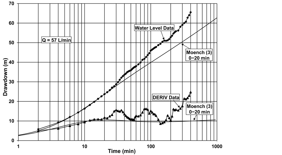
Figure 11. Test B27, semi-log plot of drawdown (Water Level Data) and logarithmic derivative (DERIV Data) for a 57 L∙min−1, 400 minutes test with the following flow regimes: Moench 3-leaky aquifer (0 - 20 min).

Figure 12. Test B743, semi-log plot of drawdown (Water Level Data) and logarithmic derivative (DERIV Data) for a 38 L∙min−1, 340 minutes test with the following flow regimes: Moench 3-leaky aquifer (0 - 55 min).
4.96 × 10⁻⁵ m2∙s−1 for Test B4 (Table 4)) and decline by more than two orders of magnitude immediately after stimulation (from T = 3.03 × 10⁻⁴ for Test B25 to 5.90 × 10⁻⁷ m2∙s−1 for Test B28 (Table 8)). Unfortunately, the results of the dos Santos et al. [3] paper could not be reproduced in the present study. Finally, the best evidence that the Moench leaky aquifer better describes the flow regime is that the T values derived from the Well B tests after hydraulic fracturing when the two wells were hydraulically connected, are nearly identical to those of the Well A tests (ratios of 1:1.0 - 1.3) and the SHF model does not fit any of the Well A test data.
4. Discussion
The sequence and order of the changes for the flow-controlling mechanism during the three pre-hydraulic fracturing tests of Well A progressed from early-time well-bore storage (first test, Test A2), through earlyto mid-time single, vertical, extended fracture (second test, Test A3), to midto late-time leaky aquifer effects (Tests A2, A3, and A5). These changes and the associated increasing T values at later times during the individual tests are probably due to the effects of well development as a result of the extensive pumping of Well A, prior to the hydraulic fracturing procedure, and the expansion of the trough of depression to an area with a higher T value. Due to the different pumping rates, analysis periods and models providing best fits to data, it is somewhat difficult to compare the changes between the three tests, but it appears that T progressively declines from one test to the next. This trend was most likely due to dewatering of the aquifer.
The Moench (Cases 1 and 3) model best fits the data from the two tests conducted immediately after hydraulic fracturing of Well A, and from the two tests of that well performed a year later (Table 9). During early time of Test A2, the drawdown and derivative plots have unit slopes typical of well bore storage effects, while leakage occurs at later times. The main advantage of the Moench model is that it considers both well-bore storage and leakage effects, while the Hantush solution neglects the effects of casing storage, which increases early drawdown, and the Papadopulos-Cooper model ignores leakage, which stabilizes late drawdowns. This may be the reason that, relative to the Moench model, the Hantush model under-estimates T values, while the Papadopulos-Cooper solution over-estimates them. The Hantush and Moench Case 1 models both assume upper and lower constant head boundaries, while the Moench Case 3 model assumes constant upper and impermeable lower boundaries. The 16 m of marine silts and clays and 6 m of weathered bedrock, consisting primarily of fine sand, found in Well B form a water table aquifer that could be the source of an upper constant head boundary. Although there are no obvious lower constant head boundaries, the discrete fractures in each well could mimic a weak constant head, so that good fits could be achieved assuming either constant head or impermeable boundaries. The weathered zone exists under water table conditions and is hydraulically coupled to locally confined bedrock. Evidence of this connection is that water levels in wells completed in bedrock follow topography and their yields vary seasonally in response to changing climatic conditions. As a result, leakage from the weathered zone to bedrock can occur, as well as dewatering of the aquifer; both factors which can affect the results of pumping tests.
dos Santos et al. [3] stated that horizontal fractures formed as a result of the hydraulic fracturing process and based their comment on a study by Murdoch and Slack [49] , which did not include the New Hampshire test site. Murdoch and Slack [49] stated that the hydraulic fractures they created were formed at shallow depths (1 - 12 m) in fine-grained sediments, nearly all of which were in glacial till or weathered formations. At various sites in the Murdoch and Slack [49] study, vertical fractures were formed as depth increased or in relatively massive sediments. Murdoch and Slack did not include fractures formed in competent bedrock at the depths described by Stewart [10] (35 - 130 m). Also, Stewart [10] indicated that most of the natural joints (fractures) in the bedrock (Exeter diorite) are steeply dipping. In some places the fractures may have gentle dips, but in the vicinity of the well sites most were inclined at steep angles.
With the exception of Test A741, the results of the dos Santos et al. [3] study could be reproduced using the Papadopulos-Cooper model, but the residual statistics suggest that there are poor fits between the observed and simulated drawdowns. For Test A741, the T value (1.55 × 10⁻⁵ m2∙s−1) obtained using the Moench (Case 1 & 3) solution in the present study is more consistent with the other post-hydraulic fracturing tests using the Papadopulos-Cooper model (T = 1.60 × 10⁻⁵ to 2.25 × 10⁻⁵ m2∙s−1) than that of dos Santos et al. [3] (T = 6.37 × 10⁻⁵ m2∙s−1) (Table 9).
Manual fitting of Barenblatt type curves for a double-porosity aquifer were used in the Stewart [10] study. Our results indicate that none of the data from the tests could fit either of the double-porosity models of Moench [23] or Barker [25] . In addition, analytical plots and derivative analyses indicated that the sigmoidal shape of the drawdown curves or depressions in the derivative curves typical of a double-porosity aquifer were not present during any of the tests.
Prior to hydraulic fracturing, the late-time T during Test A2 was 2.53 × 10⁻⁶ m2∙s−1. The early-time T from the first test (Test A14) after hydraulic fracturing was 8.29 × 10⁻⁶ m2∙s−1, which declined to 4.08 × 10⁻⁶ m2∙s−1 after
Table 9. Comparison of the best preand post-hydraulic fracturing transmissivity estimates for Wells A and B.
Note: Hantush A/S = Leaky aquifer with aquitard storage. SVF (I) = Single vertical fracture (infinite conductivity). SHF = Single horizontal fracture.
the first 30 minutes, and continued to decline to 3.16 × 10⁻⁶ m2∙s−1 during the follow-on test (Test A16). The hydraulic fracturing process probably extended the fracture in Well A into and provided a better hydraulic connection with an area having a higher T value. Hydraulic fracturing records seem to confirm this interpretation in that they suggest that a fracture was propagated early in the hydraulic fracturing process. At late-time a different zone was traversed by that fracture. The decline in T values noted in tests A14 and A16 could be due to dewatering of a shallow aquifer, possibly formed in the reported sandy portion of the surficial material overlying the bedrock in the area of Well B.
A similar pattern was noted during the two 1974 tests of Well A, except that the T values were higher. The T values derived from the Moench model were 1.55 × 10⁻⁵ m2∙s−1 during the first test (Test A741) and 7.00 × 10⁻⁶ m2∙s−1 during the second test (Test A742). One explanation for the higher T values is that long-term pumping of the well caused the trough of depression to extend into an area of even higher T values than occurred during the 1973 tests. The subsequent decline in T, again, was probably due to dewatering of the weathered zone. Unfortunately, no information concerning the post-hydraulic fracturing operational history of the well is presented in either the Stewart [10] or dos Santos et al. [3] studies.
Prior to hydraulic fracturing of Well B, the T from the first test (Test B3) was 3.25 × 10⁻⁶ m2∙s−1. The follow-on test (Test B4) produced a T = 6.38 × 10⁻⁶ m2∙s−1, an increase that could have been due to better well development, caused by extended pumping of the well (Table 9). There is no evidence of dewatering in the Test B4 data. This is probably due to either the relatively low pumping rates, masking by the effects of well development, or a combination of both factors. After hydraulic fracturing, the calculated T from the first test (Test B25) of 6.71 × 10⁻⁶ m2∙s−1 is nearly the same as that for Test B4, suggesting no significant change occurred after the hydraulic fracturing procedure. Had dewatering occurred prior to the hydraulic fracturing, this would have indicated that the T value declined immediately after stimulation. The T declines to 2.37 × 10⁻⁶ m2∙s−1 during the second test (Test B27) and, then, during the final test (Test B28) increases back to 5.42 × 10⁻⁶ m2∙s−1. In this instance, some dewatering may have occurred during Test B27 followed by expansion of the trough of depression to an area with a higher T during Test B28. The response observed during the first two tests is similar to that which occurred during the two post-hydraulic fracturing tests of Well A.
A similar pattern to the Well A results is noted during the two 1974 tests of Well B. The T obtained using the Moench model is 1.49 × 10⁻⁵ m2∙s−1 during the first test (Test B743) and 6.72 × 10⁻⁶ m2∙s−1 during the second test (Test B744). As with Well A, an explanation for the higher T values is that long-term pumping of the well caused the trough of depression to extend into an area of even higher T and the decline in T during the second test was due to aquifer dewatering. Neither of Stewart [10] or dos Santos et al. [3] provided any information concerning the post-hydraulic fracturing operational history of Well B.
A comparison of the highest T value prior to and the T value immediately after hydraulic fracturing would provide a measure of how effective the process was in each well, by eliminating or minimizing changes due to well development and aquifer dewatering. For both wells, the Moench solutions are used for consistency in making the comparisons. In the case of well A, the highest T value (late-time Test A2) prior to and the T value immediately after (Test A14) hydraulic fracturing were 2.53 × 10⁻⁶ and 8.29 ×10⁻⁶, respectively, or a factor of 3.3, which was similar to the increase in the pumping rates from 38 to 95 L∙min−1, or a factor of 2.5. There was no dewatering of fractures and water levels were relatively stable at the end of the tests, suggesting that the pumping rates may provide good approximations of the reliable yields of Well A. For Well B, there was no significant change in the T values just before and immediately after hydraulic fracturing (6.38 × 10⁻⁶ for Test B4 and 6.71 × 10⁻⁶ m2∙s−1 for Test B25). The water level did not stabilize at 15 L∙min−1 during Test B4, but was stable at the end of Test B25, while pumping at 37 L∙min−1. Primary water-bearing zones were dewatered and water levels never stabilized during each of the follow-on post-hydraulic fracturing tests of Well B, at pumping rates between 38 and 57 L∙min−1. These results indicate that the best estimate is that the yield of Well B increased from less than 15 L∙min−1 to less than 38 L∙min−1 as a result of the hydraulic fracturing process. Because there was no increase in the T after hydraulic fracturing in Well B, the increase in yield of Well B may be related to the propagation of the major fracture in Well A hydraulically connecting the two wells after hydraulic fracturing and increasing the drainage area of Well B.
Stewart [10] reported that there was no communication between Wells A and B during pumping tests conducted prior to the hydraulic fracturing procedures. During post-hydraulic fracturing tests, however, there were measurable drawdowns in the non-pumping well that occurred 30 - 60 minutes after the start of pumping. No water level data were included in Stewart [10] so the degree of interference could not be estimated. Because of this evidence that the fracture propagated from Well A and hydraulically connected the two wells, it is likely that the drainage area for Well B was increased, which could account for its increased yield. The sum of the individual yields in the previous paragraph indicate that the total change in yield of the two wells was from less than 53 L∙min−1 to less than 133 L∙min−1, a potential increase by a factor of 2.5, or about one half of the 5.3 times increase indicated by dos Santos et al. [3] . This estimate does not take into account the effects of well interference caused by the hydraulic connection between the two wells. There is insufficient information available to determine the degree of interference, but it is possible that there may have been little or no increase in the total yield of the two wells after the hydraulic stimulations were completed. It would require more extensive testing or long-term monitoring of well operations (records of daily production, hours pumped, and water levels) to determine if this were the case.
5. Summary and Conclusions
The sequential change of the flow regime during the pre-hydraulic fracturing tests of Well A is from early-time wellbore storage (first test, Test A2), through earlyto mid-time single, vertical, extended fracture (second test, Test A3), to midto late-time leaky aquifer effects (all tests). These changes and the associated progressively increasing T values are probably due to the effects of well development as a result of the extensive pumping of Well A and the extension of the trough of depression to an area with a higher T. There is an apparent progressive trend of declining T between the individual tests that is probably related to aquifer dewatering. Stewart [10] stated that most of the fractures in the vicinity of the well were steeply dipping. The Moench leaky aquifer model best fits the data from the pumping tests completed immediately after hydraulic fracturing of Well A and the tests conducted one year later. The aquifer test analyses indicate that the one prominent vertical fracture in the well was extended to an area with a higher T value by the hydraulic fracturing process. There are declines in T values during the aquifer tests conducted after hydraulic fracturing in both 1973 and 1974 [10] that are probably related to dewatering of the shallow sandy portion of the aquifer. dos Santos et al. [3] stated that T increased by 46 times after hydraulic fracturing, but the present analyses suggest the T only improved by a factor of 2.8 and that the improvement in T was due to propagation of a fracture to an area of the aquifer with a higher T.
Prior to hydraulic fracturing of Well B, the T nearly doubled between the first and second tests (Tests B3 and B4, respectively), which is probably due to better well development as a result of the extended pumping of the well. There was no evidence of dewatering, possibly due to either the low pumping rates or being masked by the effects of well development. After hydraulic fracturing, there was no immediate change in the T during the first test (Test B25), but it declined and then increased during the second test (Test B27) and third test (Test B28), respectively. One year later, the T again declined after the first test (Test B743) to a value nearly identical with the last pre-hydraulic fracturing test (Test B4), suggesting that there was no effective long-term increase in T due to the hydraulic fracturing process. This would seem to confirm the Stewart [10] observation that the geophysical logs showed no clear evidence that fractures were formed hydraulically in that well. These results differ from those of dos Santos et al. [3] who stated that the T increased in Well B by 285 times after hydraulic fracturing.
The T values after hydraulic fracturing in both Well A and Well B were nearly identical. Because there was no effective change in the T for Well B, it is probable that the primary water-bearing fracture in Well A was propagated in the direction of Well B. Both wells could have then been receiving water from the same reservoir or portion of the aquifer. After hydraulic fracturing, the sum of the individual yields of Well A and Well B increased by a factor of 2.5. However, the wells were then hydraulically connected, so that there may have been no significant increase in the total overall yield of the two wells.
After well development, the two primary flow-controlling mechanisms were leakage and dewatering of fractures. This was not evident on the log-log graphs used by Stewart [10] and the fractures could only be detected on diagnostic and derivative plots. Leakage is identified by a steady drawdown and then recovery of the derivative towards zero. Dewatering of fractures was rateand time-dependent, and produced either a constant drawdown or a peak on a derivative curve. Even with the advantage of an inverse analysis, various models could provide similar fits to specific sets of drawdown data. Application of diagnostic and derivative plots to sort out the best solutions is essential to determining the correct model to apply to a set of time-drawdown data.
Acknowledgements
We gratefully thank Christoph Butscher of the Karlsruhe Institute of Technology and Ingrid Padilla of the University of Puerto Rico for their careful review of this manuscript. Their suggestions have greatly improved our manuscript.
NOTES
*Corresponding author.