Numerical Analysis of Printed Circuit Board with Thermal Vias: Heat Transfer Characteristics under Nonisothermal Boundary Conditions ()
1. Introduction
Because of an increase in heat dissipation from electronics components placed on a printed circuit board (PCB), a thermal via has been used as one of the thermal solutions to enhance the heat transfer through the PCB. In many cases, the thermal via is a small hollow cylinder of copper, and their arrays are placed inside the board. The thermal conductivity of the metal via is about 1000 times higher than that of a dielectric material, and therefore the via serves effectively as a heat conduction path through the board.
Many studies have been published on the heat transfer characteristics of thermal vias. Lee et al. [1] conducted the analysis of thermal vias in a high density interconnect layer. A closed-form analytical model was presented using the Bessel functions. Nakayama [2] conducted a detailed analysis on the heat conduction in the PCB. This study dealt with a substrate for a ball grid array package, where a belt of densely populated through-vias and two continuous copper layers were placed. Li [3], on the other hand, addressed a simple model for the analysis of thermal vias. One-dimensional heat flow inside the PCB was assumed, and a calculation model was presented based on a thermal resistance network. Hatakeyama et al. [4] showed a two-dimensional thermal resistance network model of the thermal via. The model was verified by comparing calculation results with experimental ones. Furthermore, the effectiveness of the thermal via was shown by Guenin [5] and Kafadarova and Andonova [6] by changing the number of vias. Bissuel et al. [7] also showed the effectiveness of micro-via structures in the PCB.
In industry, thermal engineers use effective thermal conductivity for calculation of heat transfer through the PCB. The PCB is a composite board, where complicated metal wirings are placed in a dielectric material. The use of effective thermal conductivity simplifies the calculation process because the PCB can be modeled as a homogeneous medium.
Concerning the effective thermal conductivity of the PCB, the analytical studies were published by Culham and Yovanovich [8] and Shabany [9]. Culham and Yovanovich pointed out the importance of a spreading resistance as well as a metal resistance for the calculation of effective thermal conductivity. Shabany clarified the effects of a component (heat source) size and copper layers in the PCB on the evaluation of effective thermal conductivity. Moreover, Nakayama et al. [10] have launched the study to develop a scheme to estimate the effective thermal conductivity, which will be implemented into a system of computer codes.
This paper describes the numerical analysis on the heat transfer characteristics of the PCB having thermal vias. Unlike previous studies, the present analysis focuses on nonisothermal boundary conditions. Although the effect of boundary conditions on the effective thermal conductivity of the PCB was examined by Culham and Yovanovich [8] and Shabany [11], their models did not have the thermal vias. In the present analysis, under 2nd and 3rd kinds of boundary conditions, the temperature distribution and the effective thermal conductivity of the board are discussed by changing thermal design parameters. As described by Guenin [5] and Shabany [9], since a metal sheet is an important factor to dominate the heat transfer characteristics of the PCB, the metal sheets are also included in the present mathematical model.
2. Analytical Method and Nonisothermal Boundary Conditions
Numerical analysis is conducted for the simplified PCB shown in Figure 1. This model has metal vias (thermal conductivity: λv) inside a polymer board (thermal conductivity: λb) and two metal sheets (thicknesses: δts, δbs, thermal conductivities: λts, λbs) on the top and the bottom of the board. The top surface of the model is entirely heated while the bottom is entirely cooled, and the heat transfer characteristics of the model are analyzed in an x-y-z coordinate system. The temperature distribution inside the model is obtained by solving the heat conduction equation given by
 (1)
(1)
where λj is the thermal conductivity and T the temperature. The subscripts v, b, ts and bs stand for the metal via, the polymer board, the top metal sheet and the bottom metal sheet, respectively.
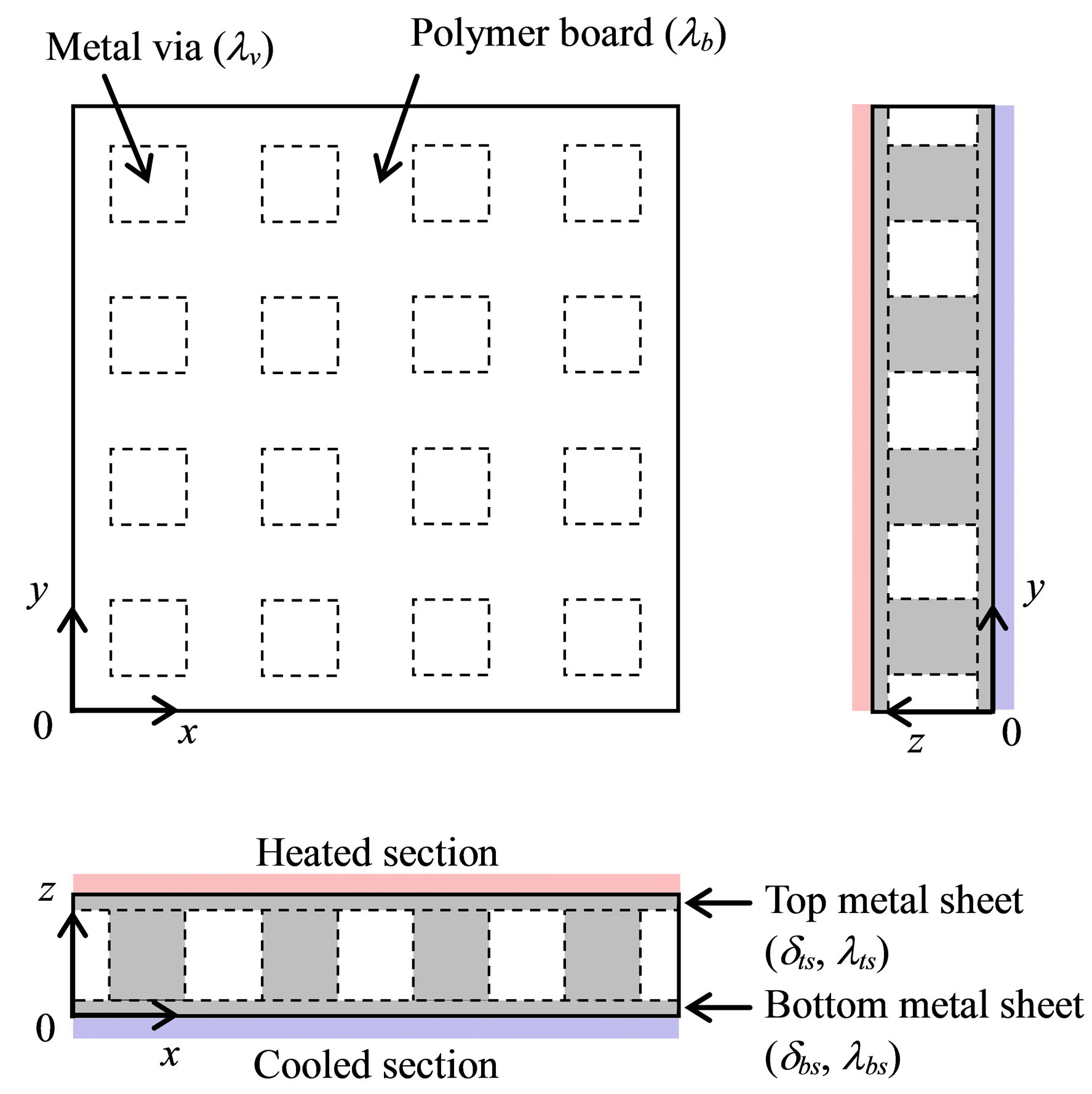
Figure 1. Mathematical model (thickness is exaggerated).
The temperature distribution and the effective thermal conductivity of the model are investigated as follows: First, the temperature distribution at the heated section (top surface) of the model is discussed under the boundary conditions of
 (2)
(2)
 (3)
(3)
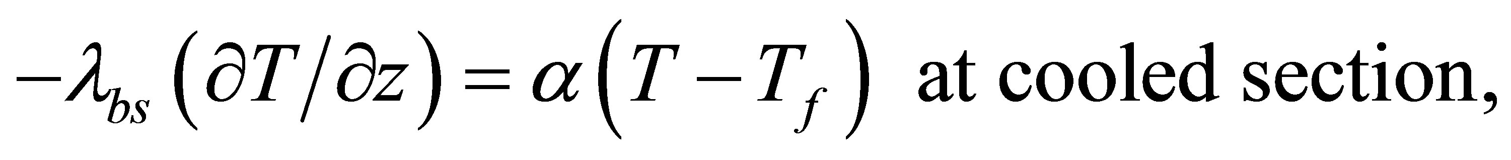
where the heat flux, qh, and the temperature, Tc, are given in calculation. Moreover, the temperature distribution at the cooled section (bottom surface) of the model is also discussed under the boundary conditions of
 (4)
(4)
 (5)
(5)
where the temperature, Th, the heat transfer coefficient, α, the cooling fluid temperature, Tf, are given.
Secondly, based on the numerical results obtained in the first investigation, the analysis is conducted on the effective thermal conductivity of the model. This discussion is made under the boundary conditions of
 (6)
(6)
 (7)
(7)
The nonisothermal boundary conditions are used at both sections.
Throughout the present analysis, the following adiabatic boundary condition is applied at the surfaces except for the heated and the cooled section:
 (8)
(8)
where n is the coordinate normal to the boundary surface.
The analysis is conducted for the board having the size of 32 mm × 32 mm × 2.0 mm (thickness). The metal via array in the board is changed as shown in Figure 2. The specification of metal vias is shown in Table 1. The metal via arrays are made keeping the total volume of vias in the board. The metal vias of Type 1 and Type 2 are too big compared with real ones; however, they are used here for comparison. Under the numerical conditions of λv = 400 W/(m·K), λb = 0.40 W/(m·K), Th = 40˚C, qh = 5.0 W/cm2 and Tc = Tf = 20˚C, the thicknesses, δts, δbs, the thermal conductivities, λts, λbs, and the heat transfer coefficient, α, are changed in the present analysis.
3. Results and Discussion
3.1. Temperature Distribution
Figure 3 shows the temperature distribution at the heated section (top surface) of the model. The numerical results are obtained under the boundary conditions of Equations (2) and (3). The three results for Type 1, Type 3 and Type 5 are compared at δts = 0.40 mm, λts = 400 W/(m×K), δbs = 0 mm (without bottom metal sheet). The temperature distribution at the cross section is also shown in this figure. Since λv is 1000 times higher than λb, the metal vias serve as main heat-flow paths through the board.

Figure 2. Schematic diagram of via arrays.
Moreover, much difference is observed between the three numerical results, and therefore it is confirmed that the temperature distribution at the heated section is strongly affected by the arrangement of metal vias.
Under the same boundary conditions as used in Figure 3, the temperature difference, ΔT, between the heated and the cooled section of the model is obtained from the numerical results. The relations between ΔT and the number of vias, N, are shown in Figures 4 and 5, where δts and λts are changed respectively at δbs = 0 mm. Because the temperature at the heated section is not uniform, the maximum and the minimum temperature difference, ΔTmax, ΔTmin, are shown in these figures. Irrespective of δts and λts, it is observed that ΔTmax decreases while ΔTmin increases slightly and therefore their difference becomes smaller with the increase in N. From Figure 4, it is found that in the cases of δts = 0.20 mm and 0.40 mm, the temperature difference is less than 2.0˚C at N = 64 (Type 4) and N = 256 (Type 5). However in the case of δts = 0 mm, a large temperature difference is still observed at N = 256. Therefore, although the metal vias are used in the board, their effectiveness is not demonstrated without the metal sheet. It is also confirmed that from Figure 5, ΔTmax and ΔTmin decrease and their difference becomes smaller with the increase in λts. This is because of the decrease in thermal resistance of the top metal sheet.
Under the boundary conditions of Equations (4) and (5), the temperature distribution at the cooled section (bottom surface) of the model is obtained as shown in Figure 6. The numerical results for Type 1, Type 3 and Type 5 are compared at δts = 0 mm (without top metal sheet), δbs = 0.40 mm, λbs = 400 W/(m×K) and α = 2000 W/(m2×K). The temperature distribution at the cross section is also shown in this figure. Furthermore, the maximum and the minimum temperature difference, ΔTmax, ΔTmin , between the heated and the cooled section of the model are shown in Figure 7 changing α as a parameter. Convective and boiling heat transfers at the cooled section are considered in this calculation. The significant influence of via population is observed not only at the heated section but also at the cooled section. Moreover, because the heat flux is not prescribed at the boundary surface, the heat transfer rate through the model is increased
 (a) (b) (c)
Figure 3. Temperature distributions at heated section and cross section (δts = 0.40 mm, λts = 400 W/(m×K), δbs = 0 mm). (a) Type 1 (N = 1); (b) Type 3 (N = 16); (c) Type 5 (N = 256).

Figure 4. Temperature difference between heated and cooled section: effect of top sheet thickness (λts = 400 W/(m×K), δbs = 0 mm).

Figure 5. Temperature difference between heated and cooled section: effect of top sheet thermal conductivity (δts = 0.40 mm, δbs = 0 mm).
 (a) (b) (c)
Figure 6. Temperature distributions at cooled section and cross section (δts = 0 mm, δbs = 0.40 mm, λbs = 400 W/(m×K), α = 2000 W/(m2×K)). (a) Type 1 (N = 1); (b) Type 3 (N = 16); (c) Type 5 (N = 256).

Figure 7. Temperature difference between heated and cooled section: effect of heat transfer coefficient at cooled section (δts = 0 mm, δbs = 0.40 mm, λbs = 400 W/(m×K)).
with α, which causes to increase ΔTmax and ΔTmin as shown in Figure 7.
From the above numerical results under Equations (2), (3) and Equations (4), (5), it is confirmed that the placement of metal sheets and the population of metal vias are important factors to dominate the temperature distribution of the model. Although the nonisothermal boundary conditions are used at the boundary surface, the temperature difference between the heated and the cooled section is almost uniform when the metal vias are populated densely with the metal sheets. In the following section, the effective thermal conductivity of the model is discussed for Type 5.
3.2. Effective Thermal Conductivity
The effective thermal conductivity, λeff, of the model is calculated by
 (9)
(9)
Under the boundary conditions of Equations (6) and (7), the value of λeff is obtained as shown in Figures 8-10. Because the temperatures at the heated and the cooled section of the model are not uniform as described above, ΔTmax and ΔTmin are used to calculate λeff, and the corresponding values of λeff,min and λeff,max are shown in these figures. Figure 8 shows the effect of δts at λts = 400 W/(m×K), δbs = 0.40 mm, λbs = 400 W/(m×K) and α = 2000 W/(m2×K). Compared with the case of δts = 0 mm (without top metal sheet), it is found that the difference between λeff,max and λeff,min for δts ¹ 0 mm (with top metal sheet) is very small, and then the difference is reduced gradually with the increase in δts. The effectiveness of

Figure 8. Effective thermal conductivity: effect of top sheet thickness (λts = 400 W/(m×K), δbs = 0.40 mm, λbs = 400 W/(m×K), α = 2000 W/(m2×K)).

Figure 9. Effective thermal conductivity: effect of top sheet thermal conductivity (δts = 0.40 mm, δbs = 0.40 mm, λbs = 400 W/(m×K), α = 2000 W/(m2×K)).

Figure 10. Effective thermal conductivity: effect of heat transfer coefficient at cooled section (δts = 0.40 mm, λts = 400 W/(m×K), δbs = 0.40 mm, λbs = 400 W/(m×K)).
metal sheet is confirmed although its thickness is several hundred microns. Figure 9 shows the effect of λts at δts = 0.40 mm, δbs = 0.40 mm, λbs = 400 W/(m×K) and α = 2000 W/(m2×K). Due to the increase in thermal resistance of the metal sheet, both λeff,max and λeff,min decrease with λts, but their difference is still small even in the case when λts is less than 10 W/(m×K). Figure 10 shows the effect of α at δts = 0.40 mm, λts = 400 W/(m×K), δbs = 0.40 mm and λbs = 400 W/(m×K). As described above, the heat transfer rate through the model is changed with α; however, it is confirmed that λeff,max and λeff,min are hardly affected by α.
The numerical analysis is also conducted under the isothermal boundary conditions expressed as
 (10)
(10)
 (11)
(11)
and then the corresponding value,  , of effective thermal conductivity is calculated by Equation (9). In this calculation, since the uniform temperatures are given at the heated and the cooled section, the temperature difference, ΔT, is simply obtained by (Th - Tc). Besides, the heat flux, qh, is calculated from the temperature gradient at the heated section. Figure 11 shows the ratio of λeff to
 , where δts is changed at λts = 400 W/(m×K), δbs = 0.40 mm, λbs = 400 W/(m×K) and α = 2000 W/(m2×K). The maximum and the minimum value,
  ,
, 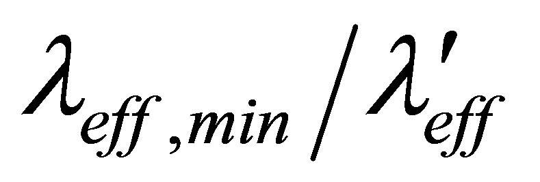 , are shown in this figure. The dashed lines are also used to indicate the difference in ±10%. Although the agreement between λeff and
  depends on the design parameters, it is confirmed that the good agreement in ±10% is obtained when the metal vias are populated densely with the metal sheets. In this case, the effective thermal conductivity is the same whether the isothermal or the nonisothermal boundary conditions are applied.

Figure 11. Comparison between isothermal and nonisothermal calculation: effect of top sheet thickness (λts = 400 W/(m×K), δbs = 0.40 mm, λbs = 400 W/(m×K), α = 2000 W/(m2×K)).
4. Conclusions
Numerical analysis is conducted on the heat transfer characteristics of the PCB, where the metal vias are placed between the metal sheets. Under 2nd and 3rd kinds of boundary conditions, the temperature distribution and the effective thermal conductivity are obtained by changing the design parameters.
From the numerical results, it is confirmed that the placement of metal sheets and the population of metal vias strongly affect the heat transfer characteristics of the PCB. Although the nonisothermal boundary conditions are applied at the boundary surface, the temperature difference between the heated and the cooled section is almost uniform when the metal vias are populated densely with the metal sheets. In this case, the effective thermal conductivity of the PCB is found to be the same whether the isothermal or the nonisothermal boundary conditions are applied.
Nomenclature
N: number of via (-)
n: coordinate normal to boundary surface (m)
q: heat flux (W/cm2, W/m2)
T: temperature (˚C)
x, y, z: coordinate (m)
Greek Symbols
α: heat transfer coefficient (W/(m2×K))
ΔT: temperature difference (K)
δ: thickness (mm)
λ: thermal conductivity (W/(m×K))
Superscript
': isothermal boundary condition
Subscripts
b: polymer board bs: bottom metal sheet c: cooled section eff: effective f: cooling fluid h: heated section max: maximum min: minimum ts: top metal sheet v: metal via