Comparison between Fourier and Wavelets Transforms in Biospeckle Signals ()
1. Introduction
When a coherent light, such as laser, illuminates a rough surface, compared the wavelength of laser, it occurs a phenomenon of optical interference with the formation of light and dark regions, called speckle [1].
After applying the dynamic surface, there is a continuous formation of new and different speckles, and these random and dynamic interference patterns is called dynamic speckle or biospeckle, if the area concerned is biological. This technique allows extracting information about the structures movement of the illuminated material, making it an interesting tool in several knowledge areas [2].
The biospeckle has been used as a technique to measure detailed extensions of pine roots [3] or even the biological activity of roots in tissue culture [4], in assessing the water activity in maize and beans seeds [5], to studies of the relationship between chlorophyll pigments present in apples and their respective biological activity [6], and several other papers.
The biological activity expressed in the context of speckle does not present a clear definition of what phenomenon is creating, however can be understood as structural and molecular motions occurring in the material analysis [4], Doppler effect, Brownian motion, variations of the refractive index [7], among others. It is a complex signal and with causes still investigated [8], which is a challenge, and at the same time, a motivation.
In this context, the use of image processing techniques and signal analysis tools can be used in the biospeckle signal to understand better this optical phenomenon.
The interference patterns analysis can use graphical methods, which generate maps indicating the spatial variability of the biological activity, or a numerical interpretation of the temporal variation of patterns formed. An alternative of the graphical and numerical classifications is a signal analysis in the time domain or in the frequency domain [5].
The analysis of biospeckle signals in the frequency domain has been an alternative for many applications, allowing the filter and images contrast, beyond search of frequency markers of phenomena that contribute to the formation of the interference patterns in time, as described by [5]. Thereby, Fourier and wavelet transforms can be a good choice to make such analysis in the frequency domain.
Several studies have been conducted using the spectral analysis in the biospeckle signal, such as [9] that used the Fourier transform to analysis bean seeds contaminated by two kinds of fungi and managed to differentiate them using the harmonics amplitude; [10] assessed damage in apples and seed germination using wavelet transform and defined frequency markers for biological phenomena, as well as [5] who studied maize and beans, and cancer isolation and others.
Although there are many papers applying spectral analysis in the biospeckle signal, the most journals use wavelet transform and there is no works evaluating if Fourier transform, which is simpler than wavelet transform. It’s enough in the frequency analysis of the dynamic speckle. In this context, the present study aims to compare the Fourier and wavelet transform in the spectral analysis of biospeckle signal.
2. Theory
2.1. Time History of the Speckle Patterns (THSP)
The biospeckle is a nondestructive optical technique based on the analysis of the variations of the laser light scattered from material, and the biological activity presented reflects the state of the investigated object [11].
Follow a set of pixels of the images speckles in the time is a method of monitoring their time variations and consequently the biological activity of the studied object, and, in this context, [12] proposed the Time History of the Speckle Patterns (THSP).
The THSP is a two dimensional image that record a certain line or column of pixels in successive moments and arrange them vertically side by side. The x axis show information about the time evolution of the selected pixels and the y axis is the spatial distribution of the interference patterns [12].
2.2. Co-Occurrence Matrix
The co-occurrence matrix was presented by [13], and expresses the number of the transitions of each THSP pixel with respect to its immediate neighbor. Equation (1) describes mathematically the co-occurrence matrix.
 (1)
(1)
which:
 is the co-occurrence matrix,
  correspond the number of occurrences of an intensity value i, followed by an intensity value j to move through rows or columns of the time history.
Phenomenon that show low biological activities, their time variations of the speckle patterns are slow and present a THSP horizontally in the elongated shape and the co-occurrence matrix is characterized by small changes of the pixels intensity to i and j, as illustrated in the Figure 1(a). However, materials that exhibit high biological activity shows fast intensity variations in the THSP that resemble an ordinary spatial speckle patterns and their co-occurrence matrix has nonzero elements near the main diagonal (Figure 1(b)) [14].
2.3. Absolute Values of the Differences (AVD)
One of the methods for analyzing of the speckle patterns is the technique of the absolute values of the differences (AVD), proposed by [15] as an alternative the inertial moment technique.
The AVD method is a statistics moment of first order which it is applied on the co-occurrence matrix and generates a number [11] which allow quantify the biological activity of the studied material. Equation (2) presents mathematically the AVD technique
 (a)
(a) (b)
(b)
Figure 1. Time history of the speckle patterns and their respective co-occurrence matrix. Materials with low (a) and high (b) biological activity.
 (2)
(2)
which:
AVD is a dimensionless value, i and j are coordinates of the row and column respectively, and Mij is called of modified co-occurrence matrix and that is presented in Equation (3).
 (3)
(3)
According [15], the inertial moment showed to be more sensitive than AVD on analyzing processes that involve high biological activities, although when this variation is not so intense, this method is less efficient.
2.4. Fourier Transform
Information of the biospeckle data in the frequency domain has been an alternative to the interpretation of the interference patterns [5], with the possibility of improve the visualization of some phenomena of the studied material and to know their spectral signatures. In this context, the Fourier transform is one of the tools that can be used to spectral analysis of the biospeckle.
Fourier transform can be understood as the mathematical technique that transforms a signal from the time domain to the frequency domain, and it is formed by a set  of orthogonal functions, of period 2π [16]. Equation (4) described mathematically the Fourier transform.
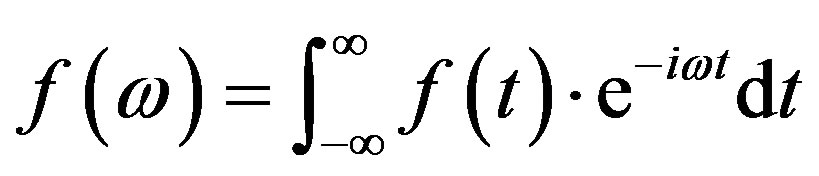 (4)
(4)
which:
 = amplitude of each component ω of the signal.
There is also the inverse Fourier transform, which is used to transform the signal from frequency domain to time domain with the reconstruction of the original function. Equation (5) presents the mathematical expression of the inverse Fourier transform.
 (5)
(5)
The Fourier transform indicates the spectral information of the signal without providing the instant which these components happen, and in situations that to know when the frequencies occur are interesting precludes the use of Fourier transforms, unless if the series is stationary [17]. In this context, the wavelet transform is an alternative that provides the instant the frequency components occur.
2.5. Wavelets Transform
The wavelets are simply waves of duration adjusted with energy concentrated in variables intervals [18], which makes it a great useful method for time series analysis, that exhibit characteristics that can change in the time and in frequency.
The continuous wavelet transform is defined as the convolution of  with a scaled and translated version of
  [19], called wavelet mother. Equation (6) describes mathematically the continuous wavelet transform.
 (6)
(6)
which:
 is the studied signal a scale parameter b translation value
 is the mother function of wavelets
 is the spectrum wavelets.
The scale is related to the frequency, in which high scales correspond to low frequencies and low scales correspond to high frequencies, whereas the translation is the displacement of the mother function about the studied signal [20].
The return of the signal from frequency domain to time domain, inverse wavelets transform, allows observe the behavior of the signal in specifics frequencies bands and also the reconstruction of the original function . According [19], the inverse wavelet transform can be realized by the sum of real part of wavelet spectrum on all scales (Equation (7)).
 (7)
(7)
which:
 is a factor that convert the wavelets transform in energy density,
 ;
; ;
; ;
;  are specific constants of the base function used.
One of the major difficulties in wavelet analysis is the identification of the scales set used in the wavelet transform. Orthogonal wavelet, there is a limit and a discrete set of scales, as given by [21], however, for analysis of non-orthogonal wavelet, can use an arbitrary scales set to build a more complete signal [19].
In this context, [19] suggested Equations (8) and (9) to calculate the scales interval to be used in the wavelet transform, in which sj is the lowest and J is the highest scale.
 (8)
(8)
 (9)
(9)
The s0 should be chosen so that the Fourier period is , and to the Morlet wavelet the largest value that can adjust the scale is
  of 0.5. For other wavelet functions can be used a larger value.
2.6. Sampling Theorem
The sampling theorem describes the relationship between sampling frequency of a signal and the frequency maximum of the reconstructed signal. Below is transcript the sampling theorem as presented by [22].
“Theorem 1: If a function  contains no frequencies higher than W cps, it is completely determined by giving its ordinates at a series of points spaced 1/2 seconds W apart”.
According to the theorem, the number of samples per unit time of a signal is called rate or frequency sampling (W), and half the sampling frequency corresponds to the frequency maximum of the signal which can be reproduced in full without aliasing error.
The sampling theorem is used in this work to define the highest frequently during the decomposition of signals.
3. Materials and Methods
It was conducted a comparison between Fourier and wavelet transforms using the time history of speckle patterns (THSP) relative to a paint drying process and presented by [23].
The database was formed by 8 THSP’s collected each 20 minutes during the paint drying using the back-scattering experimental setup. Each time history was made by a set of 128 images, resolution of 512 by 640 pixels, whose time acquisition between images was of 0.08 seconds (sampling frequency of 12.5 Hz).
The lines of the THSPs were concatenated creating a new signal that was decomposed into frequency spectra using Fourier and wavelet transforms with application posterior of the inverse transform. Some frequency bands were eliminated before the reconstruction of the signal in order to analyze the results of the speckle signal using a numerical method to measure the speckle activity. The selective filtering was conducted as well in order to create some frequency markers linked to the physical phenomena under monitoring.
According the sampling theorem the highest frequency that can be seen in the reconstruction process is 6.25 Hz, and using Equations (8) and (9) were calculated the number of frequency bands used in the transform. In addition, in the continuous wavelet transform was used mother function of Morlet, a damped complex exponential with a set of oscillation parameter that preserves an approximate relationship between the scale of the wavelet analysis and the frequency in a Fourier analysis, as described by [24].
The signal resulting of the inverse transform was converted to THSP format again and numerically analyzed using the technique of the absolute values of the differences (AVD) [15], and their values compared to the gravimetrical measurement.
Figure 2 illustrated all the methodology used.
4. Results and Discussion
Figure 3 presents the absolute value of the differences for the THSP’s of the paint drying process with decomposition and reconstruction of some frequency bands using Fourier transform.