A Comparison between Evolutionary Metaheuristics and Mathematical Optimization to Solve the Wells Placement Problem ()
1. Introduction
Consider an oil reservoir for which oil production totals over the entire reservoir area are given (or estimated). We are interested in the Wells Placement Problem (WPP), i.e., the problem of maximizing the total oil production of the reservoir by selecting locations to build at most a certain number of vertical wells at a given minimum distance apart from one another.
WPP (and variations of it) has been the subject of a number of studies in the last decades [1-9]. The main approaches used to find solutions have been Genetic Algorithms (GA), which are a special type of Evolutionary Metaheuristics, and Integer Programming (IP), a subclass of Mathematical Optimization.
To the best of our knowledge, the earliest study of wells placement optimization using IP was the work conducted in 1974 by Rosenwald and Green [8], who developed a numerical optimization framework to select optimal positions of wells. Their objective was to minimize the difference between actual and desired flow curves by choosing optimum well locations from predefined location sets. In 1997, Vasantharajan and Cullick [9] introduced the term reservoir quality to represent reservoir connectivity adjusted by tortuosity, which was the surface area surrounding the flow by the volume contained. The well site selection process was performed through IP, with the goal of maximizing reservoir quality. Later, in 1999, Cullick et al. [4] improved the formulation of the problem by reducing its number of constraints.
On the other side, GA is the most widely used method to solve WPP optimization [1]. Guyaguler et al. [6] developed a hybrid method of GA linked with polytope search and coupled with a proxy generated by kriging. The objective function in this work was to maximize net present value by finding the optimum injection well locations. The output of this work indicates that using kriging as a proxy with the hybrid optimization framework reduced the computational expense considerably. This work was extended by Badru and Kabir [2] by including horizontal wells and linking the hybrid GA with experimental design to find the impact of uncertainty on recovery and the number of wells required. In 2006, Bangerth et al. [3] compared GA with four algorithms designed to solve WPP. GA was also compared with Covariance Matrix Adaptation-Evolution Strategy by Ding [5] to optimize well locations for different types of wells with calculated productivity index as the objective function. Onwunalu et al. [7] used GA combined with statistical proxy to establish a relationship between the variables and the objective function using unsupervised learning techniques.
Some of the articles cited above report computational results using either GA or IP, but we are not aware of a study that compares both. In this paper, we use GA and IP to solve instances of WPP, and report the computational results of those tests.
Specifically, our test reservoir sits on an  grid, where each of the
  sites in the grid represents a possible location for a well. For each
 , where
  and
and , a production total
  is associated with the site, and each pair of sites chosen needs to be at least
  grid units apart from each other. Finally, the maximum number of well locations selected,
  , is predetermined.
2. Evolutionary Metaheuristics
Evolutionary Metaheuristics use ideas of biology and Darwin’s theory of evolution, such as reproduction, mutation, and “survival of the fittest”, to provide solutions to problems that arise in other fields of study. Because one of the most used types of evolutionary metaheuristics in petroleum engineering is genetic algorithms, we developed a GA to tackle our problem of interest (for details on the structure and use of GA in general, see [10]).
2.1. Definition of Terms and Variables
Our GA starts with an initial population that is improved through crossover, local search, mutation, and the addition of new members to the population, which we call intruders. After a generation, the best fit individuals of the population are selected, the others are discarded, and a new generation begins. The algorithm runs for a predetermined number of generations,  , and returns the fittest individuals of the final population. The fitness of an individual, here, is the total oil production associated with it.
An individual  is represented by an
  -array of ordered pairs (which we call coordinates), and denoted as

where ,
,  , represent the locations on the grid of the wells defined by
 . Associated with
 , the value
  is the total oil production that results from choosing this individual, given by Equation (1).
 (1)
(1)
We denote the  production totals matrix by
 , i.e., an element of row
  and column
  of
of  is
is , and we define
  We let
  be the sorted vector of the elements of
  and its corresponding coordinates:

where
 ,
,
 and
and
 .
.
2.2. The Genetic Algorithm
The high level structure of our GA is as follows:

At each generation ,
,  is the number of individuals in the initial population,
  is the number of crossover operations performed, and
  is the number of intruders created. The value
  is used in the sub-routine LOCAL-SEARCH, and will be explained later.
Lines 1 - 5 initialize the variables of the algorithm, which are the individuals of the population, at zero. Line 6 creates the initial population, and lines 7 - 12 perform evolutionary sub-routines for  generations. Finally, line 13 returns the best fit individual found.
Throughout the algorithm, and for all individuals considered, it is verified whether the distance of all locations in the grid associated with the individual satisfy the minimum distance constraint. When it does, we say that the individual is feasible. This verification is done using the following sub-routine.

This routine takes as input an individual,  , and returns 1 if the individual is feasible, or 0 otherwise. The procedure simply computes the Euclidean distance between every pair of coordinates that define the individual, and checks whether the distance is at least
 .
.

The routine INITIAL-POPULATION can be divided into two main blocks: lines 1 - 12 and 13 - 29. The first block creates a “greedy” solution to the problem by choosing the coordinates of , the first individual of the population, based on the vector
  of sorted values of
 . The second block creates the rest of the initial population by selecting random locations on the grid (using the function
 , which returns a random element of a finite set
 ), with the condition that each individual created is feasible.
We note that, for large values of , it may be hard, and perhaps even impossible, to find
  locations on the grid such that the minimum distance between each pair of locations is
 . Our algorithm makes
  attempts to find such locations, and, in the case that it is not successful, some of the coordinates of the individual being created remain as
 .
.
The sub-routine CROSSOVER performs the reproduction of individuals. In this routine, two individuals of the population  are selected at random (lines 2 - 3), and the crossover point, represented by
 , is also selected at random (line 4). In lines 5 - 12, the crossover occurs, and two new individuals are created. These new individuals are then checked for feasibility, and, in the case that they are not feasible, they are “erased” from the population by setting all of their coordinates to
  (lines 13 - 21). The procedure is repeated
  times, and the routine creates
  new individuals.

Our GA then performs a local search in the grid, in the geographical sense, to try to improve every individual of the population.

In line 2, a coordinate  of individual
  is chosen at random, and, in case it is not
 , a local search in the reservoir grid, within a square of area
  centered at
 , is performed to try to find a location in the search area such that, if substituted in place of
 , will maintain feasibility of the individual and increase its associated
  value the most. The routine performs this local search for
 , and returns their updated values.
The next genetic operator is mutation, which, again, is performed for every individual of the population .
.

This routine picks a coordinate  from individual
  at random and replaces it with another coordinate picked at random in the entire grid. If the replacement keeps
  feasible and improves the value of
 , then
  is updated; otherwise,
  remains unchanged.
Our last genetic operator, INTRUDERS, creates  individuals that enter the population “from outside”. The intention of this procedure is to add variability to the population thus far created.

This routine is similar to INITIAL-POPULATION. The main differences are in lines 2 and 6, where the choice of the coordinates of the new individuals is more selective: they are chosen among the top  values of the
  matrix. Thus, this routine brings to the population not only variability, but also members with high fitness.
Our final sub-routine selects and preserves the  best fit individuals from the entire population
 , which will become the initial population of the next generation.

The sorting procedure in line 1 is, in fact, a renumbering of the individuals  based on the values
 ,
, . As a clarifying example, suppose we give as input to this line
 ,
,  , and
, and  , with
 ,
,  , and
, and . Then the output will be
 ,
,  , and
, and . Lines 2 - 7 simply erase variables
  and keep
  which are the surviving individuals that will start a new generation. (In case
 , then there will not be another generation, and WPP-GA will return
 , the individual with the best fitness found after
  generations.)
A careful analysis of WPP-GA and its sub-routines shows that the algorithm terminates, but not necessarily with an optimal solution to the problem, i.e., an individual whose fitness is the highest possible.
3. Mathematical Optimization
Mathematical Optimization approaches quantitative problems using tools such as linear algebra, calculus, and graph theory. In a sense, it is a more sophisticated method than Evolutionary Metaheuristics, and, in practice, usually requires bigger and more structured algorithms to solve a given problem.
The main advantage of using mathematical optimization, and, in our particular case, IP, is that a solution may be proven to be optimal, as opposed to GA, which does not guarantee optimality of the best solution found.
It is common practice, in IP, to formulate problems by defining an objective function to be maximized (or minimized), subject to constraints that define the problem in question. Here, the formulation of WPP is as follow:
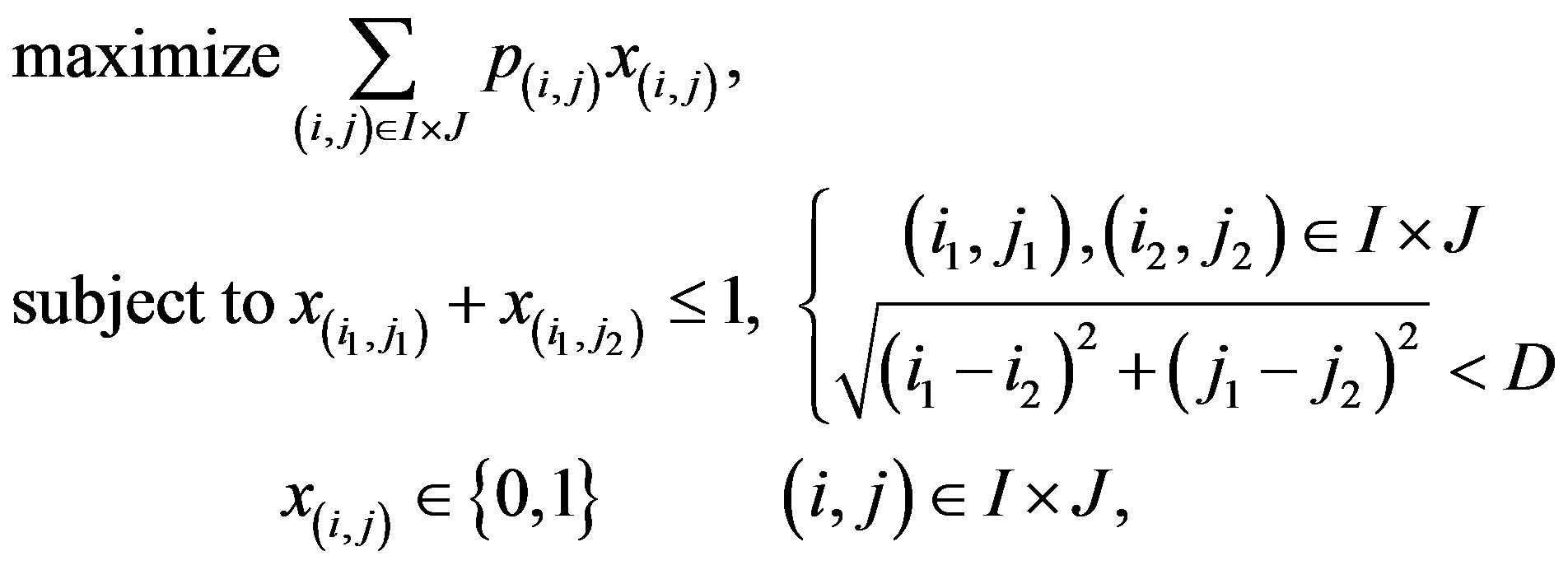
where a variable  represents the location
  in the oil reservoir grid, and is equal to 1 if the location is chosen, or 0 otherwise. Hence, a feasible solution to this problem is a
  -vector of 0’s and 1’s that satisfies all constraints defined in the formulation shown. Note that this is a completely different way of representing a solution, in comparison with our GA. Nonetheless, the values of the objective function, here, and the fitness of the individuals, in the GA, are comparable, since they have the same meaning.
To solve our instances with the IP approach, we use a commercial solver based on branch-and-cut that can handle large-scale optimization problems. For details on branch-and-cut, the reader is referred to [11].
4. Computational Tests
We ran our computational tests in the Texas Tech High Performance Computing Center’s 3.0 GHz CPUs with 16 GB RAM nodes. For the tests using IP, we used CPLEX 12 with default settings, except for the search strategy, which was set to Traditional Branch-and-Cut, and the relative and absolute gap tolerances, which were set to zero. Every test had a time limit of 3600 seconds.
Our test grid has , and we set the values of
  to
to , and
, and . For each of these values, we tried to solve WPP with
  set to
 , up to the point at which either the time limit was reached, or the value of
  was not reached, i.e., neither method was able to find a solution that represented
  well locations. For the GA, we set
 ,
,  ,
,  ,
,  , and
, and  for all tests.
The values of the  matrix were obtained with the commercial reservoir simulator Eclipse, using the Quality Maps approach (see [12] for details). Some main characteristics of our heterogeneous and anisotropic reservoir are: initial pressure of
 , porosity of 22%, and horizontal permeability average of
  with standard deviation of
 . The distance between two closest grid points is
 , and the thickness of the reservoir is
 .
.
Table 1 shows the results obtained using both GA and IP. The columns “Best Sol’ n” displays the value of the best solutions found by both methods. (Note: in GA, this value is called the fitness of the best individual, whereas in IP it is called the objective function value of the best solution. We will use the latter expression in our analysis.) “Time” shows the computational time, in seconds, required for the test to finish. We note that, because of the settings used in CPLEX, all solutions obtained using IP are provably optimal precisely when the time is less than 3600 seconds. The column “Card” shows the cardinality of the solution found, i.e., the number of well locations associated with that solution. Finally, “Gap” refers to the relative percentage difference between the GA and IP best solutions, and is computed using Equation (2).
 (2)
(2)
From Table 1, it is clear that the problem gets harder as the values of  and
and  increase. On the IP section of the table, this is reflected in the time required to solve the instances. On the GA side, both the computational time and the cardinality of the best solution show the increase in the difficulty of the problem. For instance, for
  and
and , the best solution that GA can find has cardinality 117, although solutions with greater cardinality (and better objective function value) do exist, as the IP results show.
Overall, IP was capable of finding better solutions than GA, and, most of the time, was faster. In every test, the best solution found by IP had an objective function value at least as good as the one found by the GA. In 8 cases, both methods found an optimal solution to the problem, and in 11 other cases, the gap between the two methods was less than 1%. This shows that GA can be effective for instances that are less challenging, but, for the harder instances, IP was notably more successful than GA.
The merit of being faster and finding better solutions is due not only to the differences in approaching the problem (IP vs. GA), but also a result of the algorithms used to solve the instances. While our GA has less than 500 lines of code, CPLEX is the product of professional software developers who worked on it for decades. The seemingly small values in the last columns reflect this contrast of algorithms: a gap as small as 0.1% can be very difficult to close, and thus finding a sub-optimal solution can be a much easier task than finding an optimal one. Moreover, the fact that CPLEX can guarantee the optimality of a solution is a feature that a GA does not have. It is only in comparison studies such as the present study, that one can visualize the effectiveness of a GA, in finding optimal solutions. Finally, we note that CPLEX is a multi-purpose solver that can handle a vast number of different problems, while our GA was developed specifically to tackle WPP.
5. Conclusions and Further Research
In this study, we compared the performance of GA and IP to solve instances of the problem of placing vertical wells in an  grid that sits on a reservoir, with the


Table 1. Summary of results using GA and IP.
objective of extracting the maximum amount of oil from the reservoir. Our results indicate that GA can be effective for easier instances, but it lacks performance for harder ones. In comparison, CPLEX (which takes the IP approach) always found a solution at least as good as our GA, and most of the time faster. Moreover, IP has the advantage of finding provably optimal solutions, while GA is not able to guarantee that a solution is optimal.
The GA presented here can, of course, be modified and have its performance enhanced, either by actually changing the algorithm, or by simply adjusting its parameters. Similarly, the solution via IP can be made faster by considering different formulations of the problem and tuning some parameters on CPLEX. To maintain both approaches simplely, we chose not to vary those parameters, to provide a basic GA, and to use a straightforward formulation for our IP approach.
As further research, we suggest the study of non-conventional wells placement, a more challenging problem, since it involves wells that are not necessarily vertical, and thus may require a 3D-grid as the set of possible locations for the wells.
6. Acknowledgements
The authors acknowledge the High Performance Computing Center at Texas Tech University at Lubbock for providing resources that have contributed to the research results reported within this paper. URL: http://www.hpcc.ttu.edu We thank Dr. Jerome Onwunalu’s for guidance and support, and for providing a GA code used in preliminary tests.
This research was partially supported by the Office of Naval Research (ONR) through grant N000141310041 to de Farias.