Spectral and Finite Difference Solutions of the Hyperbolic Heat Transport Equation for Thermoelectric Thin Films ()
1. Introduction
The research activity in the area of thermoelectricity began with the discoveries of Seebek, Peltier and Thomsom in the early 1800’s. Since the middle of the 1900’s there have been numerous applications of thermoelectric bulk materials resulting in cooling, heating and power generation devices. The concept of nanostructuring has revolutionized the field in the last 15 years and much investigation has been made on nanostructuring of semiconductor materials to yield quantum wells and superlattices based devices. The main effects of semiconductor nanostructuring have been on the thermal properties of the materials. In particular, superlattices made with crystalline materials appear as good thermoelectrics since they manage to scatter phonons without diminishing the electrical conductivity [1]. For this reason, superlattices of alternating materials are simple structures which improve significantly the thermoelectric properties of materials and therefore the well known thermoelectric figure-ofmerit ZT [2]. The study of irreversible processes in these thin structures is of great relevance since due to their high frequency functioning, temperature may rise reducing the life time of the device. Heat transport in the nanoscale is, however, different from that described by Fourier’s law in macrosystems. We focus in this work on the problem of heat transport in thermoelectric thin films taking into account two important features of the heat transport in the nanoscale, namely, memory and nonlocal effects and the experimentally observed reduction of the thermal conductivity in nanoscopic devices. Both may be encompassed in the framework of extended irreversible thermodynamics [3], as we will explain in Section 2. Previous works from several research groups have investigated the effect of injecting a current peak in order to optimize the performance of such thermoelectric devices [4-6]. It is worth mentioning that a proper description of heat transport in that kind of problems is not possible without including the above distinctive features of the nanoscale transport considered in this work.
The approach to solve the transport Equations is through numerical methods since they cannot be treated analytically. In general, use is made of low order numerical methods, namely, finite differences (FD). Since the non-linearity of the equation results from the source term is complemented with a Robin-type boundary condition, the FD method produces satisfying results. However, when the scale of the thermoelectric devices goes to the nanometric length scale, other effects arise, namely, the heat wave propagation or ballistic transport. When this effect is present, the classic heat transport Equation is modified by a wave Equation. It is widely known that this type of Equation is very challenging for low order methods and must be solved with a high order numerical method. In this contribution, we focus our discussion on the numerical approximations of the hyperbolic heat transport Equation on a set of discrete grid points; we shall limit our discussion to the one-dimensional problem.
We will demonstrate the application of the Spectral Chebyshev Collocation (SCC) method and compare the results obtained by the second order FD scheme and an analytic solution of the linear non-homogeneous wave Equation. The solution with the spectral method converges quickly when the number of grid points is increased. Spectral methods have been used to study heat transport based on the Maxwell-Cattaneo-Vernotte equation giving a hyperbolic transport Equation in macroscopic systems [7,8] and in some microscopic devices [9]. In Section 3, we obtain the hyperbolic Equation which will be used to describe the heat transport in the system. In Section 4 we summarize the numerical methods used to solve the transport Equation obtained in Section 3. Section 5 will be devoted to present our main results and some concluding remarks are made in Section 6.
2. Nanometric Scale Heat
The predictions of the heat transport Equation derived from Fourier law and the energy conservation Equation fit well with experimental measurements for devices with lengths much larger than the mean free path of heat carriers. However, heat transport at nanometric length scales differs from that at macroscopic scales. In the last fifteen years experiments have reported that heat flux along nanoscale is significantly lower than that predicted by the classical Fourier law. The results suggested a reduction of the thermal conductivity when the length is in the nanometric scale. These facts have motivated several efforts to improve heat transport description mainly in two directions. On the one hand, some authors have modified Fourier’s law in order to introduce nonlocal and memory effects in the transport Equation and, on the other hand, others have proposed a size dependent heat conductivity to describe adequately the drop in the heat flux when going to the nanoscale [10,11]. Reference [3] has considered nonlocal and memory effects in the framework of extended irreversible thermodynamics where heat flux and higher order fluxes are taken into account as independent variables. This scheme is formally obtained from the linearized Boltzmann Equation in the relaxation time approximation. The theory leads to a generalized thermal conductivity which depends on time and position, which in the stationary state has the following expression [12]
 , (1)
, (1)
where the relation k = 2p/L has been used in order to explore the dependence of the thermal conductivity on wave numbers k of the order of magnitude of the system’s size L (thickness). In the above expression l is the mean free path of heat carriers and K0 the bulk thermal conductivity. The thermal conductivity K, as given by Equation (1), tends to the bulk value K0 when l/L ® 0, i.e. when the system’s size is much greater than the mean free path. On the other hand, the Equation (1) describes well the drop of the thermal conductivity when L is in the order of magnitude of l as it may be seen in [12]. Another consequence of the high order fluxes scheme is a relaxation time evolution Equation for the heat flux . In the lower order this Equation takes the form of the Maxwell-Cattaneo-Vernotte Equation, which reads
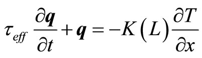 , (2)
, (2)
where teff is the effective heat flux relaxation time and T the absolute temperature. We have included the size dependence of the thermal conductivity accordingly with Equation (1) and constrained ourselves to one spatial dimension. In this work we will use Equation (2) to model the heat flux in a branch of a thermoelectric device (Figure 1) when its length goes to the nanometric scale. In this way our system becomes a thermoelectric thin film.
3. Mathematical Model
Using the heat flux, Equation (2), along with the energy conservation Equation, a single thermoelectric thin film can be modeled by a one-dimensional hyperbolic partial differential Equation,
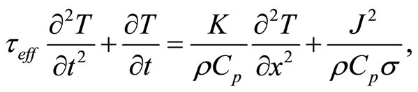 (3)
(3)
where J denotes the applied electric current density, respectively; rCp is the volumetric heat capacity; s is the electrical conductivity; whereas x and t are the spatial and temporal coordinates, respectively. The effective relaxation time teff is given in terms of the collision time tc = l/u, where u denotes the average velocity of the heat carriers [9], that is teff = tc/4. We introduce now the dimensionless variables
 (4)
(4)

Figure 1. Scheme of a thermoelectric device.
where J0 is the magnitude of the electric current through the film and Th is the fixed temperature at the hot side. Thus, dropping the asterisks, the dimensionless heat transport Equation reads
 (5)
(5)
where the dimensionless coefficients a, n and b are defined, respectively, as
 (6)
(6)
In this problem, two time scale coexist, namely, the effective relaxation scale that is given in terms of the collision time the diffusive time scale
 (7)
(7)
As it can be seen, the dimensionless coefficients and vary with the length of the system as the diffusive time scale is proportional to L. It must be noted that the thermal diffusivity is also a function of the system’s length, see Equation (1). Note that Equation (5) is valid for times between the collision and the effective relaxation time and lengths between the wave length of heat carriers and the diffusion length. The boundary conditions (in dimensionless variables) can be written as
 (8)
(8)
where the dimensionless Peltier coefficient is given by g = sJ0L/K, and s is the Seebeck coefficient. This Peltier coefficient also depends with the length of the system. The left boundary condition can be seen as a Robin-type since the temperature’s gradient is proportional to the temperature. The right (Dirichlet) boundary condition denotes the constant value at the hot side. As the initial condition, we state that the device is at room temperature (hot side temperature), that is, T(x,0) = 1.
4. Numerical Methods
Numerical simulations have been taking to treat the problem of the thermoelectric thin film. In this section we summarize the numerical methods, namely, finite differences and spectral collocation, that were used to solve Equation (5) along with the boundary conditions, Equation (8), and the initial condition stated at the end of the previous section.
4.1. Finite Differences
The code in finite differences (FD) was constructed with a forward difference scheme for the first derivative in time, while a second order central difference was applied for the second order time and spatial derivatives. Uniformly spaced grid points and constant time step were considered during the integration. The time integration was an explicit scheme. The solution was advanced in time using the second order finite difference scheme.
4.2. Spectral Chebyshev Collocation
The spectral code is based on the Spectral Chebyshev Collocation (SCC) method. This method is based on assuming that an unknown PDE solution can be represented by a global, interpolating, Chebyshev partial sum. In this spectral method, the PDE Equation is required to be satisfied exactly at the interior points, namely, the Gauss-Lobatto collocation points given by
 (9)
(9)
In Equation (9), N denotes the size of the grid. Thus, the problem is considered in a standard Chebyshev domain, that is . The derivative spatial terms of the Equation (3) were expressed on derivative matrices expanded on Chebychev polinomials. The matrixdiagonalization method was used to solve the coefficient Equation system in physical space directly. A further explanation of this spectral method can be found in [13,14]. A coordinate transformation was necessary either to map the computational interval to 0 < x < 1. In order to perform a direct comparison with the finite difference scheme, the time derivatives and the time marching were the same as the previous method.
5. Results
Figure 2(a) shows the temperature profile in the thermoelectric film when the length of the system remains in the micro-scale. We can observe that at the hot side, the temperature is the fixed temperature Th, whereas at the cold side the temperature has lowered about 3.11 degrees. The parabolic profile results from the heating Joule effect along the whole length. Figure 2(b) shows the temperature as a function of time at the cold side. As stated in section 3, at t = 0 (the initial condition), the whole thermoelectric is at room temperature, then the Peltier effect acts at the boundary reverting the heat flow and thus cooling and reducing the temperature till it reaches a steady state.
In both figures, the two numerical solutions are plotted, namely, FD and SCC. In general both solutions agree qualitatively and quantitatively in the steady state spatial distribution as well as modeling the transitory state. We define the error between both dimensionless solutions as
 (10)
(10)
The error in the steady state spatial distribution obtained
 (a)
(a) (b)
(b)
Figure 2. Comparison of the numerical schemes in the micro-scale. (a) Steady state temperature profile; (b) Transient at the cold side.
by FD approximation with N = 30 is e = 8.6 × 10⁻⁵ as with N = 10 in the SCC method, which is acceptable. However, the error in the transitory is one order of magnitude higher, that is e = 2.5 × 10⁻⁴. In both methods the time step is the same in order to perform a direct comparison since they perform the same number of iterations. Although for the case mentioned above, the speed of the SCC method is superior, this fact is not a relevant feature since the gain is less than 10%.
When L reaches the nano-scale, the wave nature of heat transfer appears clearly in the transient. This is due to the fact that the a coefficient in the heat Equation increases and the wave term becomes dominant, see Table 1. At this scale level, the Joule heating is almost not significant (b ~ 10−10). Thus, the steady state is a line with positive slope, see Figure 3(a), whereas the transient is a damped harmonic oscillation, see Figure 3(b), since the factor of the first derivative in time in Equation (3) is around the order of magnitude of the a coefficient. We must note that the coefficient n does not vary with L, it remains constant (n = p2/4). Although the FD method models the steady state correctly, the overall error is in the same order of the micro scale solution, e = 9.8 × 10⁻⁵, this error was obtained with only N = 10 collocation points for the SCC and N = 60 grid points for the FD method. Although the steady state is well-reproduced by the FD method, it does not model the transitory correctly. It shows a variation on the amplitude (e = 6 × 10⁻³) of the oscillations as well as phase difference between the two signals.
If we compare the stability conditions for both methods, in the case of pure diffusion, Dt £ Dx2/2n for FD, and for SCC Dt £ 42.55/nN4, we can infer that the spectral method requires lower time steps in order to assure stability of the solution. However, as we will see in the following, the spectral one is more robust since with less collocation points than FD the convergence of the solution

Table 1. Dimensionless coefficients as a function of the length of the system.
is assured, so that at the end we should use more grid points and smaller time steps for the FD in order to obtain low error accuracy.
Although the SCC method is more difficult to code than FD, they have many advantages: high accuracy, efficiency and exponential convergence. The trial functions of the FD are overlapping local polynomials of low order in contrast with the global smooth functions of the SCC. If we continue to decrease L the wave Equation form would arise, since the Joule effect and the Peltier effect would tend to zero, coefficients b and g, respectively, seeing the tendency of their values in Table 1. In Figure 4(a), the exact and the numerical solutions of the pure wave problem with both Dirichlet conditions, are shown at t = 0.75 with N = 1000 grid points for the FD and N = 200 collocation points for the SCC method. As it can be noted, these kinds of step-solutions solutions are very challenging numerically speaking. Numerical approximations of such nonsmooth solutions would suffer from the well-known Gibbs phenomenon. Consequently, the numerical solutions become oscillatory near the singularity and high order convergence will be lost near the singularity [15]. For the time-dependent problem, the scheme would even become unstable. Here we see that
 (a)
(a) (b)
(b)
Figure 3. Comparison of the numerical schemes in the nano-scale. (a) Steady state temperature profile; (b) Transient at the cold side.
 (a)
(a) (b)
(b)
Figure 4. Comparison of the numerical schemes for the linear wave equation. (a) Profile at t = 0.75; (b) Error of the schemes compared to the analytical solution as a function of the grid points N.
the FD numerical solution yields a small scale oscillations at both sides of the step-solution even though the stability condition Dt £ Dx/c (where c = 1, is the propagation wave speed of the wave) is not violated. That is, this condition means that the wave speed of the numeric scheme must be at least as large as the wave speed of the exact Equation. It reflects the difficulty inherent in approximating a discontinuous function. The exact solution is given in [16]. It must be noted that the Lanczos sigma Factor was used to reduce the Gibbs phenomenon presented in the analytic solution. Figure 4(a) shows the solution behaviors for both methods. In the previous figure, it is showed that the global structures of the solutions with the SC methods remain the same as the grids are refined. One would be led to believe that the oscillations could be real, however, it is found that the frequency of the oscillations is directly proportional to the number of grid points N, furthermore, the amplitude of the oscillations does not decrease much even when the grid is highly refined. In other words, these oscillations are purely numerical artifact due to the discretization of the finite grid [15].
The solutions for the wave Equation are similar in the step zone [0.4:0.6], however, different global behaviors are different for both methods, but the results with the SCC method clearly shows low overall error, see Figure 4(b). In general, the spectral methods present exponential convergence with the solution. In the presented simulations, after N = 300 collocation points, the error between the analytic and numerical approximation downs below 1 × 10⁻⁴. Such behavior has to be compared to the almost constant error of the finite-difference approximation which is relatively high.
6. Concluding Remarks
The hyperbolic heat transport partial differential Equation representing the thermoelectric problem in thin films was solved on a discrete grid system using a finite difference and a spectral collocation scheme. We have included in the model a system’s length dependent thermal conductivity to include size effects on the heat transfer. This is a novel aspect of heat transfer in the nanoscale which had not been included in other models (see for example [7,8]). At microscopic scale, both methods show comparable results, however, the error in the transient state is one order higher than in the steady state. At nanometric scale, compared to the results with the finite difference method, the spectral approximation reveals the details of dynamics of the solution with great efficiency. As the system’s length scale diminishes further more than the nanometric scale, the pure wave behavior of heat carriers appears which is described by the linear wave Equation. We have also studied the numerical issues arising in this last Equation. In this case, the finite difference scheme yields short scale oscillations, the so called Gibbs phenomenon. In contrary, the SCC method shows the so called spectral convergence with low error. This may imply that numerical solutions of the thermoelectric problem with simple finite difference schemes should be avoided when dealing with heat transfer in the nanometric length scale.
7. Acknowledgements
A. Figueroa thanks a grant from PROMEP (México). F. Vázquez acknowledges financial support from PROMEP and CONACYT (México) under grant 133763.