Variational Procedure of Deriving Diffusion Equation for Spreading in Porous Media ()
1. Introduction
The problem of deriving the governing equations of spreading matters in porous media, derived under different propositions was considered in [1-3]. Thus in [1], we thoroughly used the fact that centered Gaussian processes are completely determined by the (two points) correlation function. A multipoint correlation appears when a linear fixed-point equation is averaged. That each of these correlations splits into a finite (but increasing with the number of points) number of products of correlation functions was quite important for us. It is possible to use the diagrammatic method with more general processes [3]. Then we have much more terms in the expansions. Even if we replace the coefficients of the fixed-point equation for u by functions of a centered Gaussian process, the method is not of a simple use. It is possible to obtain similar results via a variational method, which we will explain for the example of problem, already considered in [1,2]. Not surprisingly, we then will retrieve the already obtained macroscopic equation. Then, we will use the variational method for a variant of equation including functions of a centered Gaussian process.
2. Mathematical Model
2.1. Statement of the Method
The idea goes back to so-called variational (functional) derivatives [4].
Let  be a functional over function
 . Then ratio
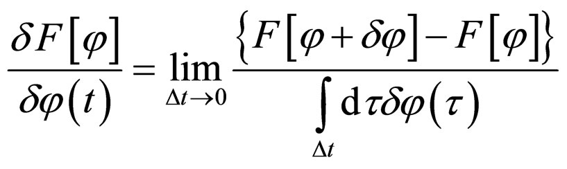
is named a variational (or functional) derivative. It is obvious that this derivative is also a functional that depends on function  and point t (as a parameter). In this way we can define the second functional derivative of
  with respect to
  at point
 :
:
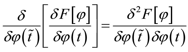 .
.
This is again a functional with respect to  that depends on the couple of parameters
  and so on.
In the case when functional 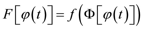 depends on functional
  (this is the most interesting case for us) the functional derivative satisfies chain rule:
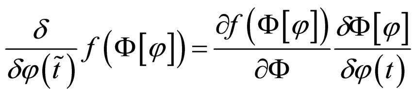 .
.
And with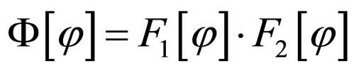 , we have
 .
.
Also notice that the functional derivative of functional  with respect to function
  satisfies
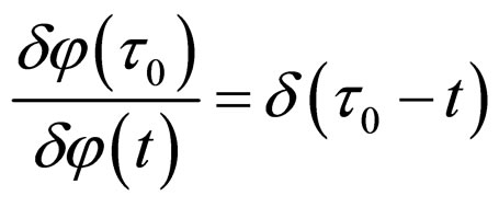 and this is very convenient for differentiation procedure.
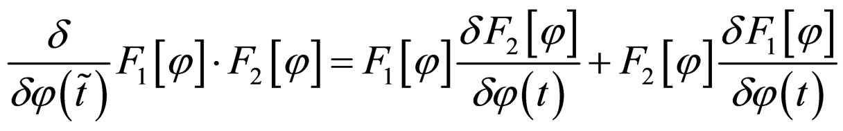
For following purposes we take the functional 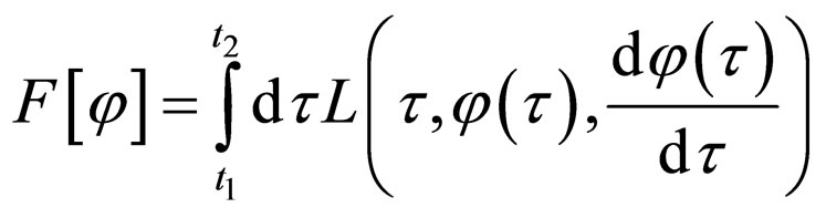 . Then we will obtainaccording to above formulas:
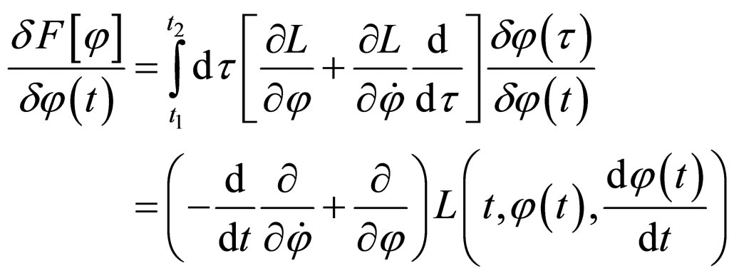
if .
.
Functional Taylor’s series for functional  over function η(τ) about a point η ≈ 0 looks like [4]:
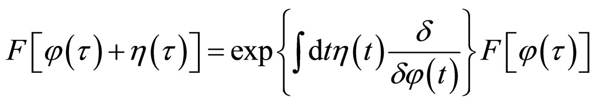 where functional shift operator
  is understood in the sense of expansion over infinite integration limits.
2.2. Application of Variational Method
In [1-3] we used the special summation procedure of diagrams of a certain type and received the diffusion equation with fractional derivatives. In this section, we will exploit another method for to receive the self-contained systems of governing equations for diffusion problems that we have used also in [5]. We again consider the spreading of matter in a porous medium such (1) rules the particles transfer on the small scale and we repeat this equation here once more:
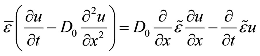 .
.
Averaging with respect to realizations  of the random porosity yields
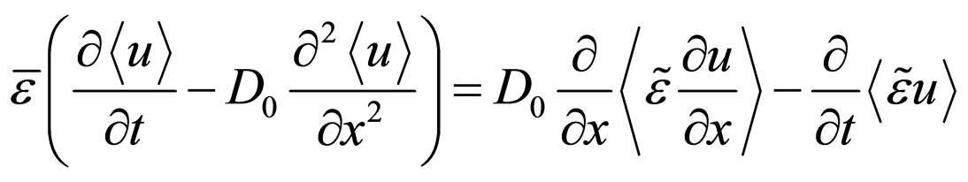 . (1)
. (1)
This equation contains the unknown , and also
 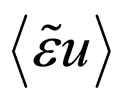 and
and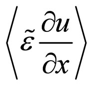 . However, the Furutsu-Novikov formula connects the new unknowns to functional derivatives of
  itself, since [4,6-8] the concentration
  is a functional of
 . Indeed, we have:
 (2.14)
Here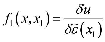 ,
, 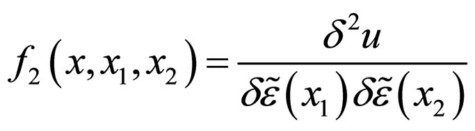 , and so on,
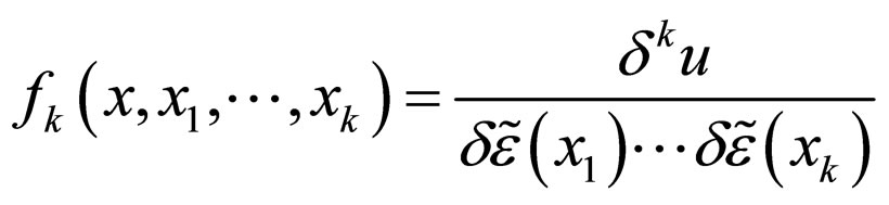 are functional derivatives of increasing order k or of functional
 , with respect to
 , at points
 . The functions
  above are cumulant of random field
 . A similar expression can also be derived for functional
  instead of
  in the equation above
 .
.
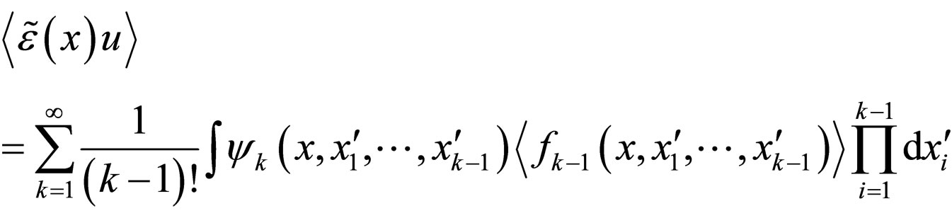
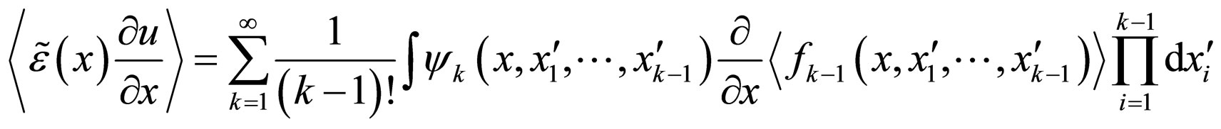
By substituting all above into (1), we derive:
We see here that together with averaged concentration  we have also averaged values of functional derivatives for
  of different orders:
 . By taking the functional derivative of (1) with respect to
  at point
 , we obtain
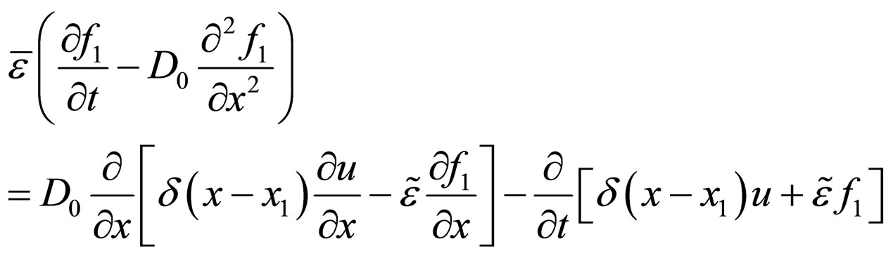 (2)
(2)
Here  in turn is a random functional
  , with two free coordinates which are
 . By averaging (2) over random realizations of
 , we receive the following equation for
 :
:
 (3)
(3)
This equation contains the unknown function  and also new unknown functions, which are
  and
and . If we apply Furutsu-Novikov formula to functionals
  and
and  instead of
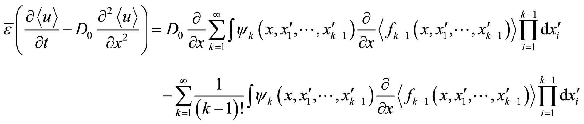
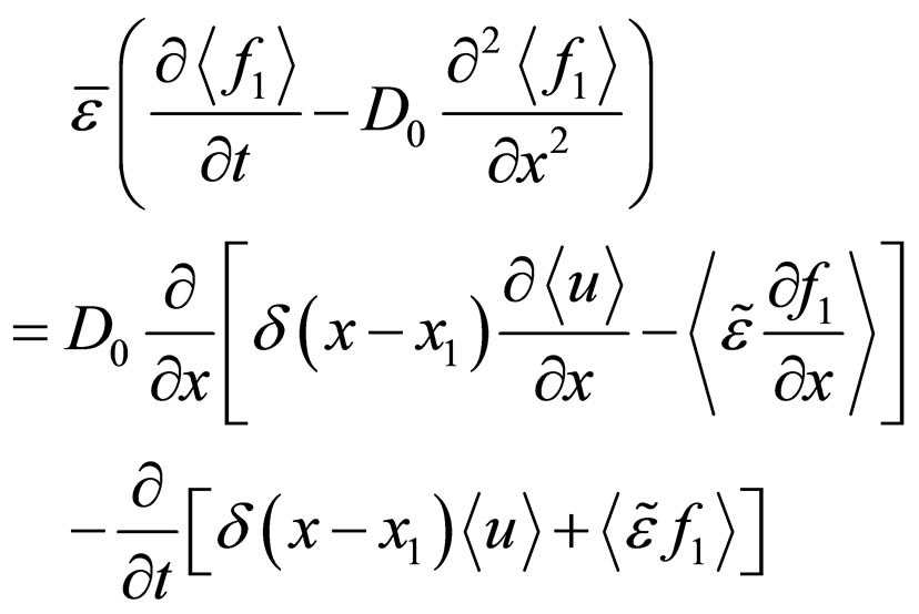
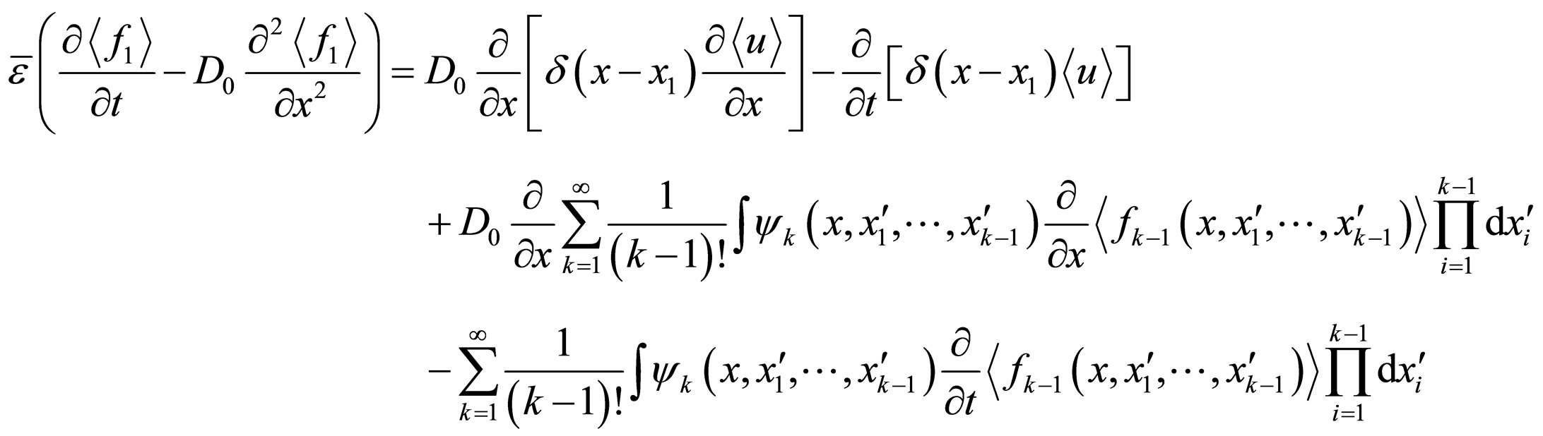
 , then substituting the results into (3), we find: (see below (4))
We should have written here “and so on”, since after that we should take the functional derivative over  and then average the obtained equations over the realizations of
  and apply Furutsu-Novikov’s formula again. As a result, we would obtain an equation for
  . Iteratively using the procedure would lead us to an infinite system of equations for the sequence of functions
 , if we set
 .
.
The structure of the thus obtained equations is such that the k-th equation in the hierarchy, with unknown  on the left hand-side has
 ,
,  , and the concentration
  in its right hand-side. And we are led to set the natural question “When can we break this chain of equations?”. It turns out that under quite reasonable assumptions, this problem can be solved.
Here we consider random media, where cumulant functions entering Equation (4) are of the even order  where
where  denotes the amplitude of the telegraph or normal random field
 . Here we should assume that in a porous media model, and due to the definition of the porosity
  we should take for granted that
 . Considering the fluctuations to be weak, we neglect cumulant of the order higher than two. Moreover, each time
  is a centered Gaussian process, all the cumulant are equal to zero, except
  which also is to the two-point correlation function of process
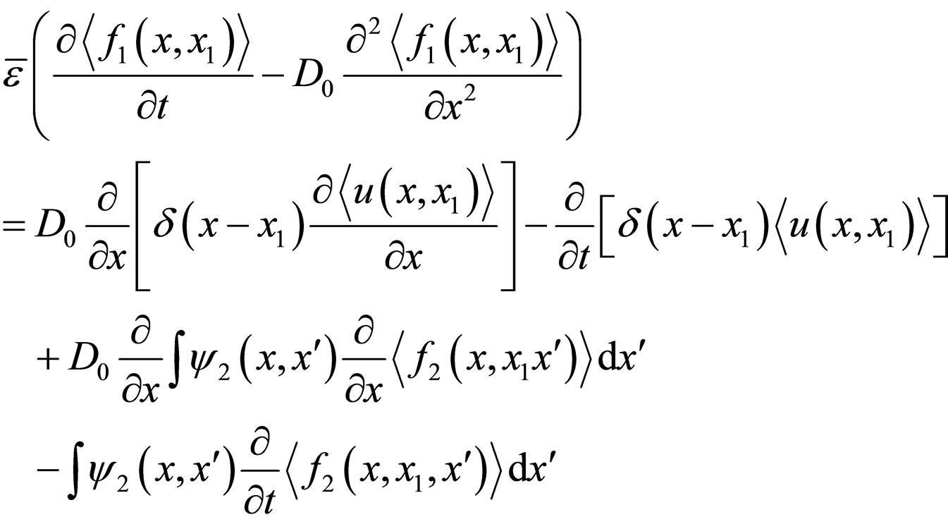
 . That is why in (4) and as well as in subsequent equations, which are not given here, we can leave only the addends containing the second order correlation functions. In this case, instead of above we get, respectively:
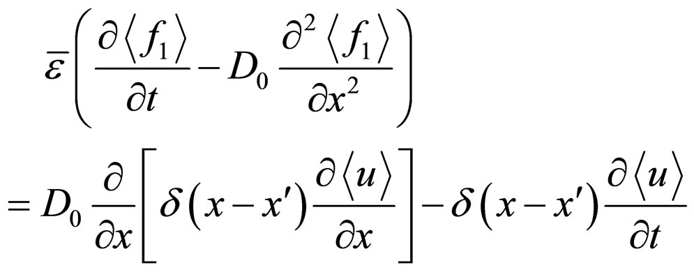
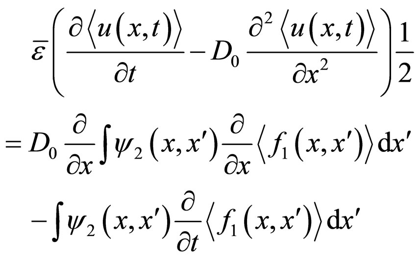
 (5)
(5)
We mentioned that if porosity represents itself a normal random field, then (5) is exact because all cumulant except one are zero. As we consider small porosity fluctuations, then in the right-hand side of (5) the third and the fourth addend in the right-hand part, containing , will be neglected because they are proportional to
 . Since also the functional derivative of
 , computed respect to
  itself at
  is
is  we arrive at the following system of equations, which turns out to be closed and has the following form:
 (6)
(6)
 (4)
(4)
 (7)
(7)
where 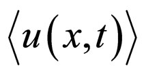 is the averaged concentration, while
 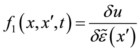 is the first functional derivative of the concentration, with respect to
 . And
. And  denotes the correlation function of second order of random field
 . System (6)-(7) will be solved in the unbounded domain
 , starting from the following initial condition:
 (8)
(8)
This leads us immediately to the following initial condition for :
:
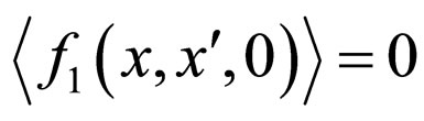 . (9)
. (9)
Indeed, we have 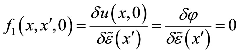 > since the initial concentration
  is determined and independent of
 .
.
In order to give the integrals on the right hand-side of (6) a concrete meaning, we now specialize the Gaussian process  by assigning a definite expression to its correlation function.
3. Basic Equation Evolution
Let us assume that the random field  is homogeneous and isotropic. Then, without any concrete definition of the correlation function
 , let us note that the latter depends only on the modulus of its arguments’ difference
 .
.
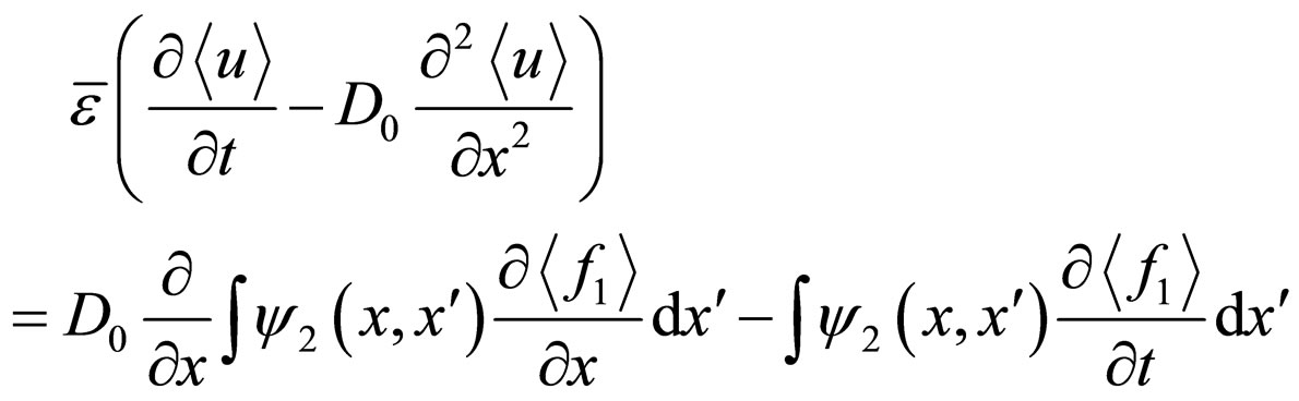
Our ultimate aim is to derive an equation related only to the mean concentration . The procedure of getting such as equation seems evident. It is clearly seen from (7) that
  are generated by the concentration that appears in the right-hand part of this equation. The function
  can be found using the Green’s function of operator
 . Then, after substituteing the obtained solution for
  into (6), we get the final integro-differential equation for
 .
.
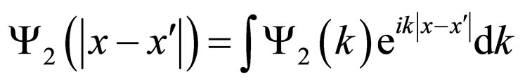
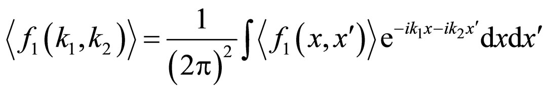
However, such a procedure is rather intricate in  - representation. In (6) and (7) it is more convenient to turn to
  -representation, i.e. to use Laplace transform with respect to time (q-parameter) and Fourier transform over with respect to space (k-parameter). After all the necessary calculations instead of (6) and (7), we get, respectively:
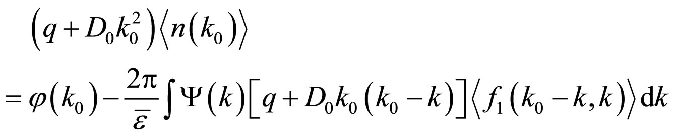 (10)
(10)
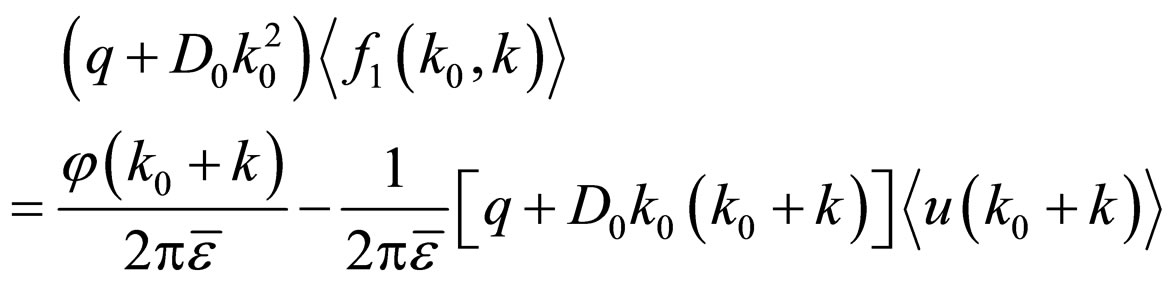 (11)
(11)
In the last relations the argument  of
of  and
and  is omitted for the sake of simplicity. We also have
and
 .
.
Also note, that if we choose  in (11) instead of argument
 , then we get the following equation for function
  appearing in (10):
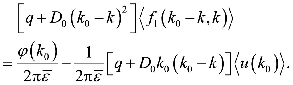
From this we compute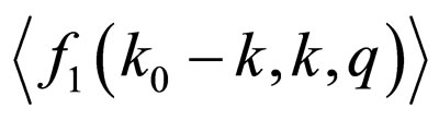 . Substituting in (10) the thus obtained expression, we get an algebraic equation with respect to
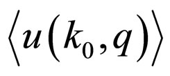 :
:
 (12)
(12)
with A and B being defined by
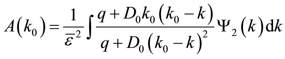 (13)
(13)
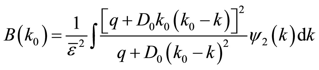 (14)
(14)
Thus, we have explicit solutions to (6) and (7) in  -representation. Therefore, Equation (12) in
  representation is equivalent to basic equation [1], which we reproduce here:
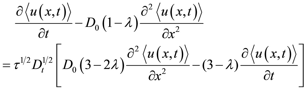 (15)
(15)
Hence successive approximation method and functional derivative method lead us to similar results for problems such that both methods are available.
4. Conclusion
So, in this paper, we presented an example of how to use the notion of a functional derivative in order to arrive at a macroscopic equation for dispersion in disordered media. In fact, we also used the present method for equation, which had been derived for a different type of disordered medium, made of inter-twisted tubes, such that a onedimensional approach has physical meaning. Hence, the example can only serve formally for two reasons. Indeed, the sample paths of Gaussian processes can take negative values, which are not good when the existence of solutions is needed. The drawback can be removed by considering ε being replaced by the exponential of a Gaussian process. We will not do it, but the presented method works fairly well for this case and gives the results already obtained via Feynman diagrams in our work [1].