The Integral of the Inverse of the Primes

Pal Doroszlai, Horacio Keller

Independent Researcher, Kékkut, Hungary.

DOI: 10.4236/apm.2023.135018                

Abstract

The present paper gives the proof of the set of primes as continuum and evaluates the analytical formula for the integral of the inverse of the primes over the distance. First it starts with the density of the primes, shortly recapitulates the prime-number-formula and the complete-prime-number-formula, the proof of the set of primes as continuum. The theoretical evaluation is followed in annexes by numerical evaluation of the theoretical results and of different constants, which represent inherent properties of the set of primes.

Keywords

Density of Primes, Prime-Number-Formula, Complete-Prime-Number-Formula, Goldbach’s Conjecture, Twin Primes, K-Tuples of Primes, Primes as Continuum

1. Introduction

For the integrability of the inverse of the primes it is a prerequisite, that the set of primes represents a continuum, meaning that the difference between adjacent primes relative to the value of the prime (distance from the origin) approaches zero.

In order to prove this prerequisite condition all steps starting with the density of the primes, their number and their distribution is shortly repeated, with reference to more detailed evaluations.

First the density of the primes as inverse of the logarithm of the distance is repeated using the fundamental identity of Riemann (see ref. [1] ), followed by the approximation of the integral of the density by summation. The error of this approximation is compensated by a recursive formula (see ref. [2] ). This involves the evaluation of a constant factor as inherent property of the set of primes.

The next step is the prime-number-formula and the proof, that this formula represents the low limit function of the number of primes, including its dispersion around of the exact value, which is evaluated with the recursive formula, given by the complete-prime-number-formula (see ref. [2] ). The standard deviation of the dispersion is proportional to the number of primes present up to the square root of the distance. The factor of proportionality is again an inherent property of the set of the primes.

The difference between the exact number of the primes over the distance and the corresponding value of the prime-number-formula is proportional to the square of the number of primes present up to the square root of the distance. The factor of proportionality is a further inherent number of the set of the primes.

The fact, that the primes represent a continuum is proved by the fact, that within an interval equal to the square root of the distance, at any distance there is at least one prime present. This is achieved by reflecting the sets of the primes over a point at any distance (see ref. [3] ), resulting the double density of occupation by the series of multiples of the primes. This reflection is used in the above reference to prove Goldbach’s conjecture and the infinity of k-tuples of primes, including twin primes.

Finally, the integral of the inverse of the primes is achieved using the analogy of the evaluation of the inverse of integers resulting Euler’s constant. The proof, that the set of the primes represents a continuum, rendering the integral of the inverse of the primes as variable is a very important fact in prime number theory.

2. Density of Primes

For the local density of positions meeting the requirement of the first constrain, the constrain of non-divisibility, the following lemma is formulated:

Lemma 2.1:

The density of primes at the distance (c) from the origin corresponds to the density of positions left free by the union of the series of multiples of the first ( $R\left(c\right)=\pi \left(\sqrt{c}\right)$ ) primes, for long distances it is approaching the inverse of the logarithm of the distance: ( $1/ln\left(c\right)$ ).

This lemma may be proven two ways:

Proof 1: The series of multiples (arithmetic progression) of any prime ( $P_{\left(n\right)}$ ) covers a subset of all positive integer positions, representing the ( $\frac{1}{P\left(n\right)}$ )-th part of all integer positions. The share of integer positions not covered by the series of multiples of each of these primes is: ( $1-\frac{1}{P\left(n\right)}$ ). The share of free positions is

multiplicative. Therefore, starting with the first prime, up to the ( $R\left(c\right)$ )-th prime the share, or density of the remaining free positions—which are not covered by the union of the series of multiples of all the first ( $R\left(c\right)$ ) primes—is given by the Euler product. For the primes this gives:

${\displaystyle \underset{n=1}{\overset{R\left(c\right)}{\prod }}\left[1-\frac{1}{P_{\left(n\right)}}\right]}$ (2.1)

The fundamental identity of Riemann (see ref. [1] ) gives, for ( $s=1$ ) the identity of Euler, with (n) running though all positive integers and considering, that at ( $c=P_{\left(n\right)}$ ) only the first ( $R\left(P_{\left(n\right)}\right)$ ) primes are covering formerly free positions is:

$\begin{array}{c}\underset{c\to \infty }{\lim }\left[{\displaystyle \underset{n=1}{\overset{R\left(c\right)}{\prod }}\left[1-\frac{1}{P_{\left(n\right)}}\right]}\right]=\underset{c\to \infty }{\lim }{\left[{\displaystyle \underset{n=1}{\overset{c}{\sum }}\frac{1}{n}}\right]}^{-1}={\left(\gamma +{\displaystyle \underset{1}{\overset{c}{\int }}\frac{1}{x}\text{d}x}\right)}^{-1}\\ =\frac{1}{\gamma +\ln \left(c\right)}=\frac{1}{\ln \left({\text{e}}^{\gamma }\cdot c\right)}=\frac{1}{\ln \left({\delta }_2\cdot c\right)}\end{array}$ (2.2)

The constant above is the Euler’s constant ( $\gamma =0.577215664901532$ ). This gives the product density of free integer positions at the distance ( $c=P\left(n\right)$ ), written with the constant of Mertens ( ${\delta }_2={\text{e}}^{\gamma }$ ) as the Euler-product.

$\underset{c\to \infty }{\lim }\left[{\delta }_2\cdot {\displaystyle \underset{j=1}{\overset{R\left(c\right)}{\prod }}\left[1-\frac{1}{P_{\left(j\right)}}\right]}\right]=\underset{c\to \infty }{\lim }{\left({\displaystyle \underset{n=1}{\overset{c}{\sum }}\frac{1}{n}-\gamma }\right)}^{-1}=\left({\displaystyle \underset{1}{\overset{c}{\int }}\frac{1}{x}\cdot \text{d}x}\right)=\frac{1}{\ln \left(c\right)}$ (2.3)

Proof 2: The Euler-product may be evaluated with the following recursions formula:

$D_{free\_Eu}\left(c\right)={\displaystyle \underset{j=1}{\overset{R\left(c\right)}{\prod }}\left[1-\frac{1}{P_{\left(j\right)}}\right]}$ ; $D_{free\_E{u}_{\left(0\right)}}=1$ ; $D_{free\_E{u}_{\left(n\right)}}=D_{free\_E{u}_{\left(n-1\right)}}\cdot \left[1-\frac{1}{P_{\left(n\right)}}\right]$ (2.4)

This recursions formula may be written as follows:

$D_{fre{e}_{\left(n+1\right)}}=D_{fre{e}_{\left(n\right)}}+\left(\frac{\text{d}}{\text{d}x}{D}_{free}\left(x\right)\right)\cdot \Delta x=D_{fre{e}_{\left(n\right)}}-\frac{D_{fre{e}_{\left(n\right)}}}{x}\cdot \Delta x$ if $\Delta x=P_{\left(n+1\right)}-P_{\left(n\right)}$ (2.5)

The total density of occupation by the union series of multiples (arithmetic progression) of all primes—following the location of the (n + 1)-th prime—is equal to the density of occupation by the series of multiples of all primes up to the location of the (n)-th prime plus the rise of the average density of occupation by the series of multiples of the (n)-th prime, if the prime ( $P_{\left(n+1\right)}$ ) is reached.

What is the analytical representation of the local density of free positions following the (n)-th prime in explicit form? To answer this question, the above recursions formula must be transformed into a differential equation and solved.

By this transformation the discrete integer variable ( $P_{\left(n\right)}$ ) must be replaced by the continuous (real) variable (x) covering the set of all positive real numbers. The density of occupation by the series of multiples of the (n)-th prime is (1/x).

The density of free positions decreases by ( $\frac{D_{fre{e}_{\left(n\right)}}}{x}\Delta x$ ) if the next primes is reached. The transformed recursions formula is the following:

$\left(\frac{\text{d}}{\text{d}x}{D}_{free}\left(x\right)\right)\cdot \Delta x=-\frac{D_{free}{\left(x\right)}^2}{x}\cdot \Delta x$ (2.6)

The differential equation of the local density of tree positions is herewith:

$\frac{1}{D_{free}{\left(x\right)}^2}\left(\frac{\text{d}}{\text{d}x}{D}_{free}\left(x\right)\right)=\frac{\text{d}}{\text{d}x}\frac{-1}{D_{free}\left(x\right)}=\frac{-1}{x}$ (2.7)

Integrated, the following solution for the logarithmically distributed “primes” is obtained:

$\frac{\text{d}}{\text{d}x}\frac{-1}{D_{free}\left(x\right)}=\frac{-1}{x}$ ; $D_{free}\left(x\right)=\frac{1}{\ln \left(x\right)+C}$ ; $C=1$ for best fitting (2.8)

Equations (2.3) and (2.8) correspond to the lemma, concluding the proof.

3. The Number of Primes

De la Valée Poussin proved 1899, (ref. [1] ), that the number of primes up to the distance (c) is given by the integral of the logarithmic density, which may be written as sum over all integers:

$\pi \left(c\right)=Li\left(c\right)+O\left(c\right)\approx {\displaystyle \underset{2}{\overset{c}{\int }}\frac{1}{\ln \left(c\right)}}\cdot \text{d}c$ ; ${\pi }_{appr}\left(c\right)\approx {\displaystyle \underset{n=2}{\overset{c}{\sum }}\frac{1}{\ln \left(c\right)}}$ (3.1)

This above sum may be written as summing up first over all integers within the sections of the length ( $\sqrt{c}$ ) and then summing up over all the ( $\sqrt{c}$ ) sections of the length ( $\sqrt{c}$ ). Taking the average value over each section and summing up over the sections is a first simplification (see Annex 2 and Annex 3), in the following used as sum over all sections:

${\pi }_{appr}\left(c\right)\approx {\displaystyle \underset{n=2}{\overset{c}{\sum }}\frac{1}{\ln \left(c\right)}}={\displaystyle \underset{j=2}{\overset{\sqrt{c}}{\sum }}\left[{\displaystyle \underset{n=\left(j-1\right)\cdot \sqrt{c}}{\overset{j\cdot \sqrt{c}}{\sum }}\frac{1}{\ln \left(n\right)}}\right]}\approx {\displaystyle \underset{j=1}{\overset{\sqrt{c}}{\sum }}\frac{\sqrt{c}}{\ln \left(j\cdot \sqrt{c}\right)}}$ (3.2)

The well proven prime-number-formula PNF results from a second simplification of the above approximation by taking for each of the sections the smallest value of the density at ( $j=\sqrt{c}$ ):

${\displaystyle \underset{j=1}{\overset{\sqrt{c}}{\sum }}\frac{\sqrt{c}}{\ln \left(j\cdot \sqrt{c}\right)}}>{\pi }_{PNF}\left(c\right)={\displaystyle \underset{j=1}{\overset{\sqrt{c}}{\sum }}\frac{\sqrt{c}}{\ln \left(\sqrt{c}\cdot \sqrt{c}\right)}}=\frac{c}{\ln \left(c\right)}=S\left(c\right)$ (3.3)

The difference between the first simplification of the number of primes and the value resulting from the PNF, (ref. [2] [3] ), is proportional to ( $R{\left(c\right)}^2=S{\left(\sqrt{c}\right)}^2$ ), the square of the number of primes up to the distance ( $\sqrt{c}$ ):

$\begin{array}{l}{\displaystyle \underset{j=1}{\overset{\sqrt{c}}{\sum }}\frac{\sqrt{c}}{\ln \left(j\cdot \sqrt{c}\right)}}-{\displaystyle \underset{j=1}{\overset{\sqrt{c}}{\sum }}\frac{\sqrt{c}}{\ln \left(\sqrt{c}\cdot \sqrt{c}\right)}}={\displaystyle \underset{j=1}{\overset{\sqrt{c}}{\sum }}\frac{\sqrt{c}}{\ln \left(j\cdot \sqrt{c}\right)}}-\frac{\sqrt{c}}{\ln \left(c\right)}\cdot {\displaystyle \underset{j=1}{\overset{\sqrt{c}}{\sum }}1}\\ ={\displaystyle \underset{j=1}{\overset{\sqrt{c}}{\sum }}\frac{\sqrt{c}}{\ln \left(j\cdot \sqrt{c}\right)}}-S\left(c\right)={\gamma }_c\cdot R{\left(c\right)}^2\end{array}$ (3.4)

because the value ( ${\gamma }_c$ ) quickly and asymptotically converges to a constant value (Annex 2):

$\begin{array}{c}{\gamma }_c=\frac{\sqrt{c}}{\ln \left(c\right)\cdot R{\left(c\right)}^2}\cdot \left({\displaystyle \underset{j=1}{\overset{\sqrt{c}}{\sum }}\frac{\ln \left(c\right)}{\ln \left(j\cdot \sqrt{c}\right)}}-\sqrt{c}\right)\\ =\frac{1}{2\cdot R\left(c\right)}\cdot \left({\displaystyle \underset{j=1}{\overset{\sqrt{c}}{\sum }}\frac{\ln \left(c\right)}{\ln \left(j\cdot \sqrt{c}\right)}}-\sqrt{c}\right)\\ =\frac{1}{R\left(c\right)}\cdot \left({\displaystyle \underset{j=1}{\overset{\sqrt{c}}{\sum }}\frac{\ln \left(\sqrt{c}\right)}{\ln \left(j\cdot \sqrt{c}\right)}}-\frac{\sqrt{c}}{2}\right)\end{array}$ (3.5)

Thus, the error of the second simplification resulting the PNF at the distance (c) is proportional to ( $R{\left(c\right)}^2$ ), the square of the number of primes present at ( $\sqrt{c}$ ). The factor of proportionality is ( ${\gamma }_c=0.28313$ ).

The relation between the error of the PNF at (c) and the square of the number of primes up to ( $\sqrt{c}$ ) is invariant. The constant factor of proportionality ( ${\gamma }_c$ ) is an inherent propriety of the number of primes.

The systematic error of the PNF may be corrected by recursive application of a correction, resulting the complete-prime-number-formula (CPNF) below, evaluated and demonstrated in ref [2] :

${\pi }_{appr}\left(c\right)={\displaystyle \underset{j=1}{\overset{\sqrt{c}}{\sum }}\frac{\sqrt{c}}{\ln \left(j\cdot \sqrt{c}\right)}}+{\displaystyle \underset{m=1}{\overset{\sqrt{c}}{\sum }}\left[{\gamma }_{sec}^m\cdot {\displaystyle \underset{j=1}{\overset{c^{\left(\frac{1}{2^{m+1}}\right)}}{\sum }}\frac{c^{\left(\frac{1}{2^{m+1}}\right)}}{\ln \left[j\cdot c^{\left(\frac{1}{2^{m+1}}\right)}\right]}}\right]}$ (3.6)

This formula converges very fast: two steps with ( $m=2$ ) are already sufficient.

The factor ( ${\gamma }_{sec}=-0.036765$ )—as an inherent property of the set of primes—is evaluated in Annex 3.

4. The Set of Primes as Continuum

The proof of the fact, that the set of primes represents a continuum is based on the proof, that within an interval equal to the square root of the distance to the origin there is always at least on prime present. If this is the case, then the difference between consecutive primes is smaller than the double value of the interval and—relative to the size of the distance—its value approaches zero with the distance growing.

For the proof, that within an interval equal to the square root of the distance there is always a prime present, the double density of occupation by the union of the series of multiples of the primes (arithmetic progression) is introduced. This double density of occupation is—as it is explained below—symmetric over the point of reflection. Consequently, if within the first interval of the length equal to the square root of the distance (c) there are primes present, then the same amount is present within the last interval of the same length just below ( $2\cdot c$ ).

Reflecting the series of multiples of any prime over a point at the distance (c) from the origin results the double density of occupation by this prime if the prime is a relative prime to (c). This, because the positions covered by the straight and the reflected series of multiples are mutually exclusive, if (c) is equal to a prime. The integer positions remaining free by the double density of occupation represent equidistant primes to the point of reflection, composing diads (see ref. [2] ). If any of the primes is dividend of the distance of the point of reflection (c), then the reflected series of multiples of this specific prime does not cover additional positions: The double density of occupation—with (c) as a prime—represents the minimum of positions left free by the double density of occupation.

The local density of free positions left by the density of occupation by the straight series of multiples of primes at the distance (d, $2<d<c$ ) below the

point of reflection is ( $\frac{1}{\ln \left(c-d\right)}$ ), by the reflected series it is ( $\frac{1}{\ln \left(c+d\right)}$ ). The

combined local density of free positions is evaluated in ref. [2] yielding with the constant ( ${\delta }_2=1.320324$ ) having the double value of the twin prime constant (C2) defined by G. H. Hardy and John Littlewood, see ref. [4] :

$D_{local}\left(c,d\right)=\frac{{\delta }_2}{\ln \left(c-d\right)\cdot \ln \left(c+d\right)}>\frac{{\delta }_2}{\ln {\left(c\right)}^2}$ (4.1)

Similarly to the evaluation of the number of primes as simplification of the integral of the local logarithmic density of primes in (3.1), the best estimate of the local density of the diads results as simplification of the integral of the above density by taking the sum over all integers (this same generalization from the primes to the twins, respectively to the k-tuples was made already by Hardy and John Littlewood):

${\pi }_{diads\_appr}\left(c\right)\approx {\displaystyle \underset{n=1}{\overset{c}{\sum }}\frac{{\delta }_2}{\ln \left(c-d\right)\cdot \ln \left(c+d\right)}}$ (4.2)

This above sum may be written as summing up first over all integers within the sections of the length ( $\sqrt{c}$ ) and then summing up over all the ( $\sqrt{c}$ ) sections analogue to (3.2). Taking the average value over each section and—as a first simplification—summing over the sections gives the best estimate value of the number of diads:

$\begin{array}{c}{\pi }_{diads\_appr}\left(c\right)={\displaystyle \underset{j=1}{\overset{\sqrt{c}}{\sum }}{\displaystyle \underset{n=\left(j-1\right)\cdot \sqrt{c}}{\overset{j\cdot \sqrt{c}}{\sum }}\frac{{\delta }_2}{\ln \left(c-n\right)\cdot \ln \left(c+n\right)}}}\\ \approx {\displaystyle \underset{j=1}{\overset{\sqrt{c}}{\sum }}\frac{{\delta }_2\cdot \sqrt{c}}{\ln \left(j\cdot \sqrt{c}\right)\cdot \ln \left(2\cdot c-j\cdot \sqrt{c}\right)}}\end{array}$ (4.3)

Similarly, to the second simplification in case of the primes in (3.3), the low limit of the best estimate number of diads results with the density taken for all sections of the length ( $\sqrt{c}$ ) at the upper limit of the sections at ( $j=\sqrt{c}$ ) the diads-number-formula (DNF):

${\pi }_{diads\_appr\_low}\left(c\right)={\pi }_{DNF}\left(c\right)={\displaystyle \underset{j=1}{\overset{\sqrt{c}}{\sum }}\frac{{\delta }_2\cdot \sqrt{c}}{\ln \left(\sqrt{c}\cdot \sqrt{c}\right)\cdot \ln \left(2\cdot c-\sqrt{c}\cdot \sqrt{c}\right)}}=\frac{{\delta }_2\cdot c}{\ln {\left(c\right)}^2}$ (4.4)

This function represents the absolute low limit of the best estimation of the number of diads at (c). This corresponds with the fact, that the standard deviation of the dispersion of the effective number of diads around its best estimate value, divided by ( $R\left(c\right)$ )—the number of primes up to ( $\sqrt{c}$ )—converges to a constant value (see ref. [2] ):

$\underset{c\to \infty }{\lim }S{D}_{\Delta \pi \_rel}\left(c\right)=\underset{c\to \infty }{\lim }\sqrt{\frac{1}{c}\cdot {\displaystyle \underset{c}{\sum }{\left(\frac{{\pi }_{diads\_appr\left(c\right)}-{\pi }_{diads\_eff\left(c\right)}}{R\left(c\right)}\right)}^2}}=0.018035$ (4.5)

Therefore, the dispersion of the effective number of diads grows proportional to ( $R{\left(c\right)}^2$ ).

It is known, that at the distance (c) the difference between the effective number of primes ( $\pi \left(c\right)$ ) and the PNF is proportional to the square of the number of primes up to ( $\sqrt{c}$ ), see (3.4) and ref. [2] :

${\pi }_{appr}\left(c\right)-S\left(c\right)={\gamma }_c\cdot {\left(\frac{\sqrt{c}}{\ln \left(\sqrt{c}\right)}\right)}^2$ with the constant ( ${\gamma }_c=0.28313$ ) (4.6)

This identity allows to state, that the difference between the best estimate number of diads and the DNF is greater, than the distance (c) divided by the square of the logarithm of the distance ( $\ln {\left(c\right)}^2$ ), multiplied by a constant ( $4\cdot {\delta }_2\cdot {\lambda }_c=1.49524$ ):

$\begin{array}{c}\Delta {\pi }_{diads}\left(c\right)={\pi }_{diads\_appr}\left(c\right)-{\pi }_{diads\_low}\left(c\right)\\ >{\displaystyle \underset{j=1}{\overset{\sqrt{c}}{\sum }}\frac{{\delta }_2\cdot \sqrt{c}}{\ln \left(c\right)\cdot \ln \left(2\cdot c-j\cdot \sqrt{c}\right)}}-\frac{{\delta }_2\cdot c}{\ln {\left(c\right)}^2}\end{array}$ (4.7)

Because of symmetry of the double density of occupation and with (4.2) follows:

$\Delta {\pi }_{diads}\left(c\right)=\frac{{\delta }_2}{\ln \left(c\right)}{\displaystyle \underset{j=1}{\overset{\sqrt{c}}{\sum }}\frac{\sqrt{c}}{\ln \left(j\cdot \sqrt{c}\right)}}-\frac{{\delta }_2\cdot c}{\ln {\left(c\right)}^2}=\frac{{\delta }_2}{\ln \left(c\right)}\cdot {\pi }_{appr}\left(c\right)-\frac{{\delta }_2\cdot c}{\ln {\left(c\right)}^2}$ (4.8)

With (4.7) follows:

$\begin{array}{c}\Delta {\pi }_{diads}\left(c\right)=\frac{{\delta }_2}{\ln \left(c\right)}\cdot \left(S\left(c\right)+{\gamma }_c\cdot R{\left(c\right)}^2\right)-\frac{{\delta }_2}{\ln {\left(c\right)}^2}\\ =\left(\frac{{\delta }_2\cdot c}{\ln {\left(c\right)}^2}+\frac{{\gamma }_c\cdot {\delta }_2\cdot c}{\ln {\left(c\right)}^2}\right)-\frac{{\delta }_2\cdot c}{\ln {\left(c\right)}^2}=4\cdot {\gamma }_c\cdot {\delta }_2\cdot \frac{c}{\ln {\left(c\right)}^2}\end{array}$ (4.9)

The DNF (4.4) taken at ( $\frac{\sqrt{c}}{2}$ ) gives the number of diads within the first section of the length ( $\sqrt{c}$ ). Because of symmetry in case of the double density of occupation the same amount of diads is present within the last section at ( $2\cdot c-\frac{\sqrt{c}}{2}$ ) of the same length and they are growing to infinity:

${\pi }_{diads\_appr\_last}\left(c\right)=\frac{{\delta }_2\cdot \frac{\sqrt{c}}{2}}{\ln {\left(\frac{\sqrt{c}}{2}\right)}^2}=\frac{2\cdot {\delta }_2\cdot \sqrt{c}}{\ln {\left(\frac{\sqrt{c}}{4}\right)}^2}$ (4.10)

If in case of the double density of occupation at ( $2\cdot c-\sqrt{c}$ ) the number of free positions within the last section of the length ( $\sqrt{c}$ ) is rising without limit to infinity, then this is certainly the case as well within the larger distance of the length () and even more in case of the single density of occupation.

The same is the case within the section of the length ( $\sqrt{2\cdot c}$ ) following ( $2\cdot c$ ), respectively within the section of the length ( $\sqrt{2\cdot c}$ ) following (c). This, because the first free position covered by the series of multiples of the smallest possible

prime greater then ( $P_{\left(R\left(c\right)\right)}$ ), equal to ( $P_{\left(R\left(c+1\right)\right)}$ ) is already greater than ( $c+\sqrt{c}$ ).

This smallest prime must be ( $P_{\left(R\left(c\right)+1\right)}\ge \sqrt{c}+1$ ) in case ( $P_{\left(R\left(c\right)\right)}$ ) and ( $P_{\left(R\left(c\right)+1\right)}$ ) are twins. In this case ( $P_{\left(R\left(c\right)+1\right)}\ge \sqrt{c}+1$ ) and the square of this smallest possible prime is already over ( $c+\sqrt{c}$ ):

$\begin{array}{c}{\left[P_{\left(R\left(c\right)+1\right)}\right]}^2={\left[P_{\left(R\left(c\right)\right)}+1\right]}^2={\left[P_{\left(R\left(c\right)\right)}\right]}^2+4\cdot P_{\left(R\left(c\right)\right)}+4\\ \ge {\left(\sqrt{c}-1\right)}^2+4\cdot \left(\sqrt{c}-1\right)+4\\ =c-2\cdot \sqrt{c}+1+4\cdot \sqrt{c}-4+4\\ =c+2\cdot \sqrt{c}+1>c+\sqrt{c}\end{array}$ (4.11)

Herewith the low limit of free positions left within the section of the size ( $\sqrt{c}$ ) following (c) is not smaller, than the number of free positions within the last section of the same size just below (c).

It follows, that the set of the primes up to ( $P_{\left(R\left(c\right)\right)}$ ) normed with this last prime represent—as limit—is a continuum, since for any prime within the set the following limit is valid:

$\frac{P_{\left(p+1\right)}-P_{\left(p\right)}}{P_{\left(p\right)}}<\frac{P_{\left(p+1\right)}+2\cdot \sqrt{P_{\left(p\right)}}+1-P_{\left(p\right)}}{P_{\left(p\right)}}=\frac{2\cdot \sqrt{P_{\left(p\right)}}+1}{P_{\left(p\right)}}<\frac{3}{\sqrt{P_{\left(p\right)}}}$ (4.12)

$\underset{p\to \infty }{\lim }\frac{3}{\sqrt{P_{\left(p\right)}}}=0$ and herewith: $\underset{p\to \infty }{\lim }\frac{P_{\left(p+1\right)}-P_{\left(p\right)}}{P_{\left(p\right)}}=0$

The knowledge of the function of the exact value of the number of the primes allows for the evaluation of the standard deviation of the effective number of the primes around the exact function, given in ref [2] . From the constancy of the relative value of the standard deviation follows the integrability on the inverse of the primes.

Additionally, the following facts prove the infinity of the number of primes within the last section:

One of the proofs of the infinity of the number of primes states, that there is always a new prime, since the product of all known primes plus one is certainly not divisible by any of the known primes.

But the number equal to the product of all known primes less one is certainly another prime too. The two neighboring positions to the product of all known primes are twin primes. Their number is therefore infinite as well.

5. The Integral of the Inverse of the Primes

With (4.12) the set of the series of multiples of all primes up to ( $P_{\left(R\left(c\right)\right)}$ ) normed with even this last prime represents—as limit—a continuum. As an analogy for the integrability of the inverse of the primes the integral of the inverse of the integers giving the formula of Euler may be taken:

$\underset{q\to \infty }{\lim }{\displaystyle \underset{n=1}{\overset{q}{\sum }}\frac{1}{n}}={\displaystyle \underset{1}{\overset{{\text{e}}^{\gamma }\cdot q}{\int }}\frac{1}{x}\cdot \text{d}x}=\ln \left({\text{e}}^{\gamma }\cdot q\right)=\gamma +\ln \left(q\right)$ ; $\gamma =0.5772156649015329$ (5.1)

The value of the Euler constant accounts for the surface difference between the analytical function and the stair function corresponding to the summation, as shown in the figure below, with (q) an integer and (x) a real variable. The surface below the lower stair function of the harmonic series is obviously always smaller than the surface below the analytical function (1/x) see Figure 1. This difference accounts for ( $\gamma$ ).

In case of the primes a similar corresponding relation may be evaluated. Compared with the harmonic series, the surface between two primes the surface is smaller:

$\frac{1}{P_{\left(p+1\right)}}<{\displaystyle \underset{r=P_{\left(p\right)}}{\overset{P_{\left(p+1\right)}}{\sum }}\frac{1}{r}}<\ln \left(P_{\left(p+1\right)}\right)-\ln \left(P_{\left(p\right)}\right)$ (5.2)

Thus ( $\frac{1}{r}$ ) must be replaced by ( $\frac{1}{r\cdot \ln \left(r\right)}$ ) in the integral. Relation (5.1) may be written for the primes—with the constant ( ${\gamma }_P$ )—as follows:

$\begin{array}{c}{\displaystyle \underset{pp=1}{\overset{p}{\sum }}\frac{1}{P_{\left(pp\right)}}}={\displaystyle \underset{P_{\left(1\right)}}{\overset{{\left[P_{\left(1\right)}\right]}^{{\gamma }_P}}{\int }}\frac{1}{r\cdot \ln \left(r\right)}\text{d}r}={\gamma }_P+\ln \left(\ln \left(P_{\left(p\right)}\right)\right)\\ =\ln \left({\text{e}}^{{\gamma }_P}\cdot \ln \left(P_{\left(p\right)}\right)\right)=\ln \left(\ln \left(P_{\left(p\right)}^{e^{{\gamma }_P}}\right)\right)\end{array}$ (5.3)

The constant ( ${\gamma }_P=1.261503$ ) is evaluated in Annex 6, again an inherent property of the set of primes.

Figure 1. Comparison of the contribution of the surface between two consecutive primes to the integral of the inverse of the real variables, resp. of the inverse of the primes.

The sum of the inverse of the primes approaches slowly a final value. The dispersion is decreasing with the distance, but for the evaluation of its standard deviation a larger set of primes should be used, as in the present paper.

Annexes

Annex A1: Definition of Vectors and Variables for the Numeric Evaluation

First some general functions and values are defined: Based on the requirement of the constrain of non-divisibility by all smaller primes, a set of consecutive primes is evaluated and written to a file. From this file they are read: ( $P=\text{READPRN}\left("\text{Primes}\_\text{large}\text{.prn}"\right)$ , $P_{\left(0\right)}=1$ ).

The number of the primes in the set and their numbering are: ( $N_P=rows\left(P\right)-1$ , $N_P=5003713$ , $n=1,2,\cdots ,N_P$ ).

The complete-prime-number-formula CPNF is evaluated with the following routine (floor and ceil stand for round down and round up):

$\exp \_\left(x\right):={\text{e}}^X$ ; ${\gamma }_{sec}=-0.036765$ : $c\_\exp \left(c,m\right):=\exp \_\left(\frac{1}{2^{m+1}}\right)$ (A1.1)

For the evaluation of the number of the next smaller prime to the distance (c) the routine ( $n_{next}\left(c,n_{last}\right)$ ) resulting the index (n) of the prime next to any integer is needed ( $P_{\left(n\right)}\le c<P_{\left(n+1\right)}$ ). The evaluation starts either at the last evaluated index ( $n_{last}$ ), or at the index resulting from the complete-prime-number-formula (see A1.1 and ref. [2] ). This, to shorten some of the evaluation processes. In case ( $P_{\left(n\right)}$ ) is greater than the distance, the index is lowered. In case it is smaller, the index is risen until the corresponding prime is just smaller, or equal to the distance:

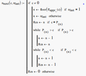(A1.2)

Further functions are the formula evaluating the index of the next smaller prime to any distance and to the square root of any distance.

$S_{eff}\left(c\right)=n_{next}\left(c,1\right)$ ; $R_{eff}\left(c\right)=n_{next}\left(\sqrt{c},1\right)$ ; $S\left(c\right)=\frac{c}{\ln \left(c\right)}$ ; $R\left(c\right)=\frac{\sqrt{c}}{\ln \left(\sqrt{c}\right)}$ (A1.3)

For the visualization of the results of the analysis the functions will be taken at sparse values, at distances corresponding to multiples of the square root of the largest prime considered.

$\Delta {\Delta }_{sp}=floor\left(\sqrt{P_{\left(N_P\right)}}\right)$ ; $k_{limit}=floor\left[\frac{P_{\left(N_P\right)}}{\Delta {\Delta }_{sp}}\right]-2$ ;

$k=1,2,\cdots ,k_{limit}$ ; $c_{s{p}_{\left(k\right)}}=k\cdot \Delta {\Delta }_{sp}$ (A1.4)

The vectors of the indexes of the primes next smaller to these sparse distances ( $P_{\left(n_{s{p}_{\left(k\right)}}\right)}<c_{s{p}_{\left(k\right)}}<P_{\left(n_{s{p}_{\left(k+1\right)}}\right)}$ ), respectively to their square root ( $P_{\left(n_{s{p}_{\left(k\right)}}\right)}<\sqrt{c_{s{p}_{\left(k\right)}}}<P_{\left(n_{s{p}_{\left(k+1\right)}}\right)}$ ), are evaluated as ( $n_{sp}\left(c\right)$ ) respectively as ( $n_{sp}\left(\sqrt{c}\right)$ ). They are evaluated once and written to files. They are read from these files:

${\pi }_{s{p}_{\left(k\right)}}=n_{next}\left[c_{s{p}_{\left(k\right)}},1\right]$ ; ${\pi }_{sqr\_s{p}_{\left(k\right)}}=n_{next}\left[\sqrt{c_{s{p}_{\left(k\right)}}},1\right]$ (A1.5)

$\text{WRITEPRN}\left("\text{index\_distance\_sp}\text{.prn}"\right)={\pi }_{sp}$ ;

${\pi }_{sp}=\text{REDPRN}\left("\text{index\_distance}-\text{sp}\text{.prn}"\right)$

$\text{WRITEPRN}\left("\text{index\_distance\_sqr\_sp}\text{.prn}"\right)={\pi }_{sqr\_sp}$

${\pi }_{sqr\_sp}=\text{REDPRN}\left("\text{index\_distance}-\text{sqr\_sp}\text{.prn}"\right)$

Annex A2: Evaluation of the Number of Primes as Sum over Sections

The number of primes as sum over sections is evaluated with (3.2) as a first simplification:

${\pi }_{sec\_appr}\left(c\right)={\displaystyle \underset{j=1}{\overset{floor\left(\sqrt{c}\right)}{\sum }}\frac{\sqrt{c}}{\ln \left(j\cdot \sqrt{c}\right)}}$ (A2.1)

The number of primes resulting from the second simplification (3.3) results the PNF. The difference between the first and the second simplification results the error of the PNF. At the instance (c) it is proportional to ( $R{\left(c\right)}^2$ ), the square of the number of the series of multiples of primes, which are covering positions at the distance (c). The factor of proportionality is evaluated over the distance as follows:

$\begin{array}{c}{\gamma }_{c\_appr\_}\left(c\right)=\frac{{\pi }_{sec\_appr\_}\left(c\right)-S\left(c\right)}{R{\left(c\right)}^2}\\ =\left[{\displaystyle \underset{j=1}{\overset{\sqrt{c}}{\sum }}\frac{\sqrt{c}}{\ln \left(j\cdot \sqrt{c}\right)}-\frac{c}{\ln \left(c\right)}}\right]\cdot \frac{\ln \left(\sqrt{c}\right)}{\sqrt{c}}\cdot \frac{1}{R(\; c\; )}\end{array}$

$=\left[{\displaystyle \underset{j=1}{\overset{\sqrt{c}}{\sum }}\frac{\ln \left(\sqrt{c}\right)}{\ln \left(j\cdot \sqrt{c}\right)}-\frac{\sqrt{c}}{2}}\right]\cdot \frac{1}{R(\; c\; )}$

${\gamma }_{c\_appr{\_}_{\left(k\right)}}=\frac{1}{R\left(c_{s{p}_{\left(k\right)}}\right)}\cdot \left[{\displaystyle \underset{j=1}{\overset{ceil\left(\sqrt{c_{s{p}_{\left(k\right)}}}\right)}{\sum }}\frac{\ln \left(\sqrt{c_{s{p}_{\left(k\right)}}}\right)}{\ln \left(j\cdot \sqrt{c_{s{p}_{\left(k\right)}}}\right)}-\frac{1}{2}\sqrt{c_{s{p}_{\left(k\right)}}}}\right]$ (A2.2)

The factors are evaluated once and written to a file. They are read from this file:

$\text{WRITEPRN}\left("\text{gamma\_c\_appr\_sp}\text{.prn}"\right)={\gamma }_{c\_appr\_}$

${\gamma }_{c\_appr\_}=\text{REDPRN}\left("\text{gamma\_c\_appr\_sp}\text{.prn}"\right)$

The factors are approaching a constant value:

${\gamma }_{c\_appr}={\gamma }_{c\_appr\_}{}_{\left(k_{limit}\right)}=0.28313$

as illustrated in Figure A2.1.

The approximating function is evaluated at sparse distances, respectively at the next smaller prime to these distances ( $P_{\left(n_{s{p}_{\left(k\right)}}\right)}<c_{s{p}_{\left(k\right)}}<P_{\left(n_{s{p}_{\left(k+1\right)}}\right)}$ ) with (2.2).

They are evaluated as well at the square roots of these distances. The evaluation at the next smaller prime corresponding to each distance assures, that the evaluated numbers of the primes correspond exactly to the distances considered:

${\gamma }_{sec\_app{r}_{\left(k\right)}}={\gamma }_{sec\_appr\_}\left[P_{\left[{\pi }_{s{p}_{\left(k\right)}}\right]}\right]$ ; ${\gamma }_{sqr\_sec\_appr\_}\left[P_{\left[{\pi }_{sqr\_s{p}_{\left(k\right)}}\right]}\right]$ (A2.3)

They are evaluated once and written to files. They are read from these files:

$\text{WRITEPRN}\left("\text{pr\_sec\_appr\_sp\_t}\text{.prn}"\right)={\pi }_{sec\_appr}$ ;

${\pi }_{sp}=\text{REDPRN}\left("\text{index\_distance}-\text{sp}\text{.prn}"\right)$

$\text{WRITEPRN}\left("\text{pr\_sqr\_sec\_appr\_sp\_t}\text{.prn}"\right)={\pi }_{sqr\_sec\_appr}$

${\pi }_{sqr\_sec\_appr}=\text{REDPRN}\left("\text{pr\_sqr\_sec\_appr\_sp\_t}\text{.prn}"\right)$

Figure A2.1. Relation of the error of the prime-number-formula to the square of the number of the series of multiples of primes, which are covering positions, over the distance.

Annex A3: Evaluation of the Factor of Correction of the First Simplification

The result of the first simplification (3.2) giving the sum over the sections of the density of primes has an error. This error is proportional to the number of primes up to ( $\sqrt{c}$ ). The error relative to ( $\pi \left(\sqrt{c}\right)$ ) results the factor of correction. Assuming the factor of correction ( ${\gamma }_{sec}$ ) is constant over the distance (c), it may be evaluated as relation of the average error to the effective number of primes ( $\pi \left(\sqrt{c}\right)={\pi }_{s{p}_{\left(k\right)}}$ ). The average error is:

$\Delta {\pi }_{se{c}_{\left(k\right)}}={\pi }_{sec\_app{r}_{\left(k\right)}}-{\pi }_{s{p}_{\left(k\right)}}$ ; $\Delta {\pi }_{sec\_a{v}_{\left(k\right)}}=\frac{1}{k}\cdot {\displaystyle \underset{j=1}{\overset{k}{\sum }}\left[\Delta {\pi }_{se{c}_{\left(k\right)}}\right]}$ (A3.1)

The value of the factor of correction is herewith:

${\gamma }_{sec}\left(c\right)=\frac{\Delta {\pi }_{sec\_av}\left(c\right)}{\pi \left(\sqrt{c}\right)}$ ; ${\gamma }_{sec{\_}_{\left(k\right)}}=\frac{\sqrt{2}\cdot \Delta {\pi }_{sec\_a{v}_{\left(k\right)}}}{{\pi }_{sqr\_sec\_app{r}_{\left(k\right)}}}$ ; ${\gamma }_{sec}={\gamma }_{sec{\_}_{\left(k.limit\right)}}=-0.036765$ (A3.2)

Figure A3.1 shows the independence of the factor of correction ( ${\gamma }_{sec}$ ) from the distance. The averaging process (A3.1) to evaluate the factor of correction is therefore justified. This factor ( ${\gamma }_{sec}=-0.036765$ ) is invariant, an inherent property of the prime numbers. It is important because it is applied in the recursive formula of the complete-prime-number-formula CPNF.

Figure A3.1. Convergence of the relation of the average relative error of the first simplification (3.2) to the final constant value ( ${\gamma }_{sec}$ ).

Annex A4: Evaluation of the CPNF and the Error of the Second Simplification

The results of the CPNF are evaluated with (A1.1) once at sparse values of the distance ( $c_{s{p}_{\left(k\right)}}$ ), written to a file are read from this file:

${\pi }_{app{r}_{\left(k\right)}}={\pi }_{appr\_}\left[P_{\left[{\pi }_{s{p}_{\left(k\right)}}\right]}\right]$ (A4.1)

$\text{WRITEPRN}\left("\text{Pi\_appr\_sp}\text{.prn}"\right)={\pi }_{appr}$ ; ${\pi }_{appr}=\text{REDPRN}\left("\text{Pi\_appr}-\text{sp}\text{.prn}"\right)$

Figure A4.1 indicates that the standard deviation of the dispersion of the effective number of primes around its approximation is rising proportionally to ( $R\left(c\right)$ ), the number of the series of multiples of primes, which are covering integer positions at this distance (c). The dispersion of the evaluated values relative to the effective number of primes at ( $\sqrt{c}$ ) is about constant over the distances up to (c): There is no systematic error.

Figure A4.1. The relative dispersion of the difference between the effective number of primes and its value evaluated with the complete-prime-number-formula (CPNF) and the relation of the error of the PNF to ( $R{\left(c\right)}^2$ ).

$\Delta {\pi }_{appr\_re{l}_{\left(k\right)}}=\frac{{\pi }_{app{r}_{\left(k\right)}}-{\pi }_{s{p}_{\left(k\right)}}}{R_{eff}\left[c_{s{p}_{\left(k\right)}}\right]}$ (A4.2)

With the results of the CPNF the factor of the proportionality ( ${\gamma }_{c\_appr}$ ) of the error of the PNF relative to the square of the number of primes present up to ( $\sqrt{c}$ ) evaluated in (A1.2) with (3.4), is reevaluated with the more exact difference as illustrated in Figure A4.1:

${\gamma }_c\left(c\right)=\frac{{\pi }_{appr}\left(c\right)-S\left(c\right)}{R{\left(c\right)}^2}$ ; ${\gamma }_{c_{\left(k\right)}}=\frac{{\pi }_{app{r}_{\left(k\right)}}-S_{\left[c_{s{p}_{\left(k\right)}}\right]}}{R_{\left[c_{s{p}_{\left(k\right)}}\right]}{}^2}$ ; ${\gamma }_c={\gamma }_{c{\_}_{\left(k_{limit}\right)}}=0.28313$ (A4.3)

Annex A5: Evaluation of the Standard Deviation of the Dispersion of the Effective Number of Primes around the CPNF

The standard deviation SD of the relative dispersion (4.5) is evaluated as follows:

$S{D}_{\Delta \pi \_appr\_re{l}_{\left(k\right)}}=\sqrt{\frac{1}{k}\cdot {\displaystyle \underset{j=1}{\overset{k}{\sum }}\frac{{\left[{\pi }_{app{r}_{\left(j\right)}}-{\pi }_{s{p}_{\left(j\right)}}\right]}^2}{R_{eff}{\left[c_{s{p}_{\left(j\right)}}\right]}^2}}}$ (A5.1)

The results are evaluated once and written to a file. They are read from this file:

$\text{WRITEPRN}\left("\text{SD\_}\Delta \text{prime\_sqr\_appr\_rel}\text{.prn}"\right)=S{D}_{\Delta \pi \_appr\_rel}$

$S{D}_{\Delta \pi \_appr\_rel}=\text{REDPRN}\left("\text{SD\_}\Delta \text{prime\_sqr\_appr\_rel}\text{.prn}"\right)$

The average of the relation of the standard deviation converges to a final value, to the factor of proportionality (). This factor is evaluated as follows:

$S{D}_{\Delta \pi \_appr\_rel\_a{v}_{\left(k\right)}}=\frac{1}{k}\cdot {\displaystyle \underset{j=1}{\overset{k}{\sum }}S{D}_{\Delta \pi \_appr\_re{l}_{\left(k\right)}}}$ (A5.2)

The results are evaluated once and written to a file. They are read from this file:

$\text{WRITEPRN}\left("\text{SD\_}\Delta \text{prime\_sqr\_appr\_rel\_av}\text{.prn}"\right)=S{D}_{\Delta \pi \_appr\_rel}\_av$

$S{D}_{\Delta \pi \_appr\_rel}\_av=\text{REDPRN}\left("\text{SD\_}\Delta \text{prime\_sqr\_appr\_rel\_av}\text{.prn}"\right)$

The constant factor is equal to the final average value of the standard deviation at large distances. The figure below illustrates that the standard deviation is about constant over the distance. This fact rectifies taking the average over the whole distance for the evaluation:

$F_{SD\_\Delta \pi }=S{D}_{\Delta \pi \_appr\_rel\_a{v}_{\left(k_{limit}-1\right)}}=0.160989$ (A5.3)

Figure A5.1 indicates that the standard deviation of the dispersion of the effective number of primes around its approximation is rising proportionally to ( $R\left(c\right)$ ), the number of the series of multiples of primes, which are covering integer positions at this distance (c). The factor of proportionality ( $F_{SD\_\Delta \pi }$ ) is again an inherent property of the prime numbers.

Figure A5.1. Dispersion of the standard deviation of the dispersion of the number of primes around its average, the resulting constant value ( $F_{SD\_\Delta \pi }$ )

Annex A6: Evaluation of the Constant of Integration and of the Dispersion of the Sum of the Inverse of the Primes around Its Approximation

The value of the constant ( ${\gamma }_P$ ) is evaluated the following way with the sum of the inverse of the primes:

${\pi }_{invers{e}_{\left(n\right)}}={\displaystyle \underset{p=1}{\overset{n}{\sum }}\frac{1}{P_{\left(p\right)}}}$ ; $S_{sum\_P\_invers{e}_{\left(0\right)}}=1$ ; $S_{sum\_P\_invers{e}_{\left(n\right)}}=S_{sum\_P\_invers{e}_{\left(n-1\right)}}+\frac{1}{P_{\left(n\right)}}$ (A6.1)

The results are evaluated once and written to a file. They are read from this file:

$\text{WRITEPRN}\left("\text{sum\_prime\_inverse}\text{.prn}"\right)=S_{sum\_P\_inverse}$

$S_{sum\_P\_inverse}=\text{REDPRN}\left("\text{sum\_prime\_inverse}\text{.prn}"\right)$

The sum of the inverse of the primes gives for the largest prime considered ( $P_{\left(N_P\right)}$ ) the value of the constant ( ${\gamma }_P$ ):

${\gamma }_P=S_{sum\_P\_invers{e}_{\left(N_P\right)}}-\ln \left[\ln \left[P_{\left(N_P\right)}\right]\right]=1.261503$ (A6.2)

For the graphical representation the evolution over the distance of the constant at sparse indexes is:

$nn=2,102,\cdots ,N_P$ ; ${\gamma }_{P{\_}_{\left(nn\right)}}=S_{sum\_P\_invers{e}_{\left(nn\right)}}-\ln \left[\ln \left[P_{\left(nn\right)}\right]\right]$ (A6.3)

The value of the constant ( ${\gamma }_P$ ) converges in fact to a final value, as illustrated in the Figure A6.1 below.

Figure A6.1. The difference of the sum of the inverse of the primes and its approximation, resulting the constant of the integral.

Conflicts of Interest

The authors declare no conflicts of interest regarding the publication of this paper.

References

[1]	Titchmarsh, E.C. (1986) The Theory of the Riemann Zeta-Function. Oxford University Press, New York.
[2]	Doroszlai, P. and Keller, H. (2022) The Number of Primes. Advances in Pure Mathematics, 12, 81-95. https://doi.org/10.4236/apm.2022.122008
[3]	Doroszlai, P. and Keller, H. (2022) The Symmetric Series of Multiples of Primes. Advances in Pure Mathematics, 12, 160-177. https://doi.org/10.4236/apm.2022.123014
[4]	Hardy, G.H. and Littlewood, J.E. (1923) Some Problems of “Partitio Numerorum” III. On the Expression of a Number as a Sum of Primes. Acta Mathematica, 44, 1-70. https://doi.org/10.1007/BF02403921