The Magnetic Field as Trigger for Disturbances of a Flow of a Newtonian Fluid through a Cylindrical Pipe with a Horizontal Axis

Ibrahima Kama^*, Mamadou Lamine Sow, Cheikh Mbow

Department of Physics, University Cheikh Anta Diop (UCAD), Dakar, Senegal.

DOI: 10.4236/mme.2022.124006                

Abstract

A Fourrier Petrov Galerkin spectral method is described for high accuracy computation of linearized dynamics for flow in a circular pipe. The code used here is based on solenoidal velocity variables. It is written in FORTRAN. Systematic studies are presented on the dependence of eigenvalues and other quantities on the axial and azimuthal wave number; the reynolds’ number Re and a new none-dimensional number Ne. The flow will be considered stable if all the real parts of the eigenvalues are negative and unstable if only one of them is positive.

Keywords

Newtonian Fluids, Magnetic Field, Linear Stability, Petrov-Galerkin, Generalized Eigenvalue Problem

1. Introduction

The flows in the pipes are presented in several industrial applications such as heat exchangers, chemical rectors, gas turbine cooling and heating systems and combustion chambers or mixing systems.

Magnetic body forces act on all materials but are generally very weak for paramagnetic and diamagnetic materials. These forces derive from a specific magnetic energy acquired by the material in the presence of an applied magnetic field.

The effects of intense magnetic fields on matter are indeed multiple and arouse the curiosity of researchers. Quantum [1], thermodynamic [2], mechanical [3] [4] effects that are imperceptible at low fields are observed in matter under strong magnetic fields. The term magneto-science is sometimes used to group together all the fields application.

One of the fields of magneto-science is the study of fluids under intense magnetic fields. The outstanding applications generally concern magnetohydrodynamics and magnetic levitation. In the first case, the fluid is necessarily driver. Currents that flow through fluid placed in magnetic fields intense generate Laplace forces allowing the movement of the fluid. In the second case, the fluid used has no magnetic or electrical properties particular. Volume magnetic forces created by magnetic devices make it possible to locally compensate for gravity and thus to maintain in levitation a fluid over a given volume.

The magnetic volume force can act on the flow of the liquid provided that the term associated with the volume forces is of the same order of magnitude as the other terms of the equation. We carry out a dimensionless study of this problem to show that it is possible to act on the flow of the fluid which we consider as being Newtonian and not conductive.

Existing superconducting devices that act on dia- or paramagnetic non-conductive liquids are system designs for magnetic levitation. They most often result from a problem of inverse synthesis: starting from a desired force field (the uniformity of the force field over the largest volume is often the greatest objective), the magnetic field is determined as well as associated magnetic field sources. We are interested in the effects that volumetric forces can have on the flow of a fluid and more particularly on the stability of the flow of such a fluid.

The objective of this work is to study the nature of the instabilities introduced by the presence of a magnetic field.

2. Equations Governing the Flow and Study Strategy

To fully account for the effects generated by the stress of magnetic actions, we will first consider the flow of Newtonian fluid in absence of magnetic field. The equations governing such flow are given by the system below.

$\{\begin{array}{l}divu=0\\ \rho \left\{{\partial }_{t}u+\left(u\cdot \nabla \right)u\right\}=-\nabla p+\eta \Delta u+\rho g\end{array}$ (1)

Secondly, we apply a surface and ortho-radial current density to the surface of the cylinder ( $j=j\cdot e_{\theta }$ ). Assuming that the stress of the magnetic actions has a longitudinal component, one can imagine a modification of the velocity $u$ and pressure p fields such as $u_m=u+u^{\prime }$ et $p_m=p+p^{\prime }$ The equations governing this new flow are as follows:

$\{\begin{array}{l}div{u}_m=0\\ divB=0\\ \rho \left\{{\partial }_t{u}_m+\left(u_m\cdot \nabla \right)u_m\right\}=-\nabla p_m+\eta \Delta u_m+\rho g+\frac{\chi }{{\mu }_0}\nabla \left(\frac{B^2}{2}\right)\end{array}$ (2)

By subtracting from this system, that satisfied by the Newtonian fluid not subjected to any magnetic field, it comes:

$\{\begin{array}{l}div{u}^{\prime }=0\\ divB=0\\ \rho \left\{{\partial }_t{u}^{\prime }+\left(u^{\prime }\cdot \nabla \right)u^{\prime }+\left(u\cdot \nabla \right)u^{\prime }+\left(u^{\prime }\cdot \nabla \right)u\right\}=-\nabla p^{\prime }+\eta \Delta u^{\prime }+\frac{\chi }{{\mu }_0}\nabla \left(\frac{B^2}{2}\right)\end{array}$ (3)

In order to generalize the study to several situations, we introduce the dimensionless parameters

$\tilde{p}=\frac{p}{\rho u_0^2};\tilde{u}=\frac{u}{u_0};\tilde{r}=\frac{r}{R};\tilde{z}=\frac{z}{R};\tilde{t}=\frac{t{u}_0}{R};\tilde{\nabla }=R\nabla ;\tilde{B}=\frac{B}{B_0}$ (4)

By replacing each variable by its expression in the previous system, we obtain the following dimensionless equations:

$\{\begin{array}{l}div{\tilde{u}}^{\prime }=0\\ div\tilde{B}=0\\ \rho \left\{{\partial }_t{\tilde{u}}^{\prime }+\left({\tilde{u}}^{\prime }\cdot \nabla \right){\tilde{u}}^{\prime }+\left(\tilde{u}\cdot \nabla \right){\tilde{u}}^{\prime }+\left({\tilde{u}}^{\prime }\cdot \nabla \right)\tilde{u}\right\}=-\tilde{\nabla }{\tilde{p}}^{\prime }+\frac{1}{Re}\tilde{\Delta }{\tilde{u}}^{\prime }+\frac{1}{Ne}\tilde{\nabla }\left(\frac{{\tilde{B}}^2}{2}\right)\end{array}$ (5)

$Re=\frac{\rho u_{0}R}{\eta }$ (6)

is the Reynolds’ number. It is the ratio of inertia effects to viscous effects.

$Ne=\frac{\chi B_0^2}{\rho \mu u_0^2}$ (7)

is a dimensionless quantity, ratio between the magnetic effects and the effects of inertia.

Consider the dimensionless number defined by

$Ka=Ne\times Re=\frac{\chi R{B}_0^2}{\eta {\mu }_0{u}_0}$ (8)

This number then represents the ratio between the magnetic effects and the viscous effects. System (5) can then be written as follow:

$\{\begin{array}{l}div{\tilde{u}}^{\prime }=0\\ div\tilde{B}=0\\ {\partial }_t{\tilde{u}}^{\prime }=-\left[\left({\tilde{u}}^{\prime }\cdot \nabla \right){\tilde{u}}^{\prime }+\left(\tilde{u}\cdot \nabla \right){\tilde{u}}^{\prime }+\left({\tilde{u}}^{\prime }\cdot \nabla \right)\tilde{u}\right]+\frac{1}{Re}\tilde{\Delta }{\tilde{u}}^{\prime }+\tilde{\nabla }\left(\frac{1}{Ne}\left(\frac{B^2}{2}\right)-\nabla {\tilde{p}}^{\prime }\right)\end{array}$ (9)

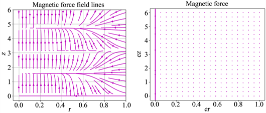
Evaluation of the Stress of Magnetic Effects

The fluid being neither charged nor conductive, we have the relation

$rotB=0$ (10)

knowing that

$B=rotA$ (11)

$A$ being the vector potential.

$rot\left(rotA\right)=grad\left(divA\right)-\Delta A=0$ (12)

We are using a stationary current distribution here. The Lorenz’s gauge condition entails

$divA=0$. (13)

We can then determine $A$ using the relation

$\Delta A=0$. (14)

The solenoid is considered very thin, it’s radius R and the surface current density is of the form

$j\left(z\right)\cdot e_{\theta }=J_0\sin \left(k_{0}z\right)\cdot e_{\theta }$ (15)

The problem is invariant by rotation around $e_z$. The magnetic and mechanical quantities therefore only depend on r and z. any plane containing $e_z$ and $e_r$ is an antisymmetry plane. The potential vector $A$ is perpendicular to the antisymmetry planes and will therefore be according to $e_{\theta }$ only. We will denote it $A_{\theta }$. The magnetic field belongs to the antisymmetry planes and will consequently have components according to $e_r$ and $e_z$.

In cylindrical coordinate

$\Delta A_{\theta }=0\Rightarrow \frac{{\partial }^2{A}_{\theta }}{\partial r^2}+\frac{{\partial }^2{A}_{\theta }}{\partial z^2}+\frac{1}{r}\frac{\partial A_{\theta }}{\partial \theta }-\frac{A_{\theta }}{r^2}=0$ (16)

as $B=rotA$

$B=-\frac{\partial A_{\theta }}{\partial z}\cdot e_r+\frac{1}{r}\frac{\partial \left(r{A}_{\theta }\right)}{\partial r}\cdot e_z$ (17)

We will denote by “int” the inside of the solenoid and by “ext” the outside.

The continuity of the normal component of the magnetic field at $r=R$ is written:

${\left(\frac{\partial {\left(A_{\theta }\right)}_{int}}{\partial z}\right)}_{r=R}={\left(\frac{{\left(\partial A_{\theta }\right)}_{ext}}{\partial z}\right)}_{r=R}$ (18)

The discontinuity of the tangential component of the magnetic field at $r=R$ imposes

$\left(B_{int}-B_{ext}\right)\cdot e_z={\mu }_0{J}_0\sin \left(k_{0}z\right)$ (19)

The vector potentials inside and outside the solenoid are respectively in the form:

We will notice in the following that:

That is

$r^2\frac{{\partial }^2{A}_{int}}{\partial r^2}+r\frac{\partial A_{int}}{\partial r}-\left(k_0^2{r}^2+1\right)A_{int}=0$ (20)

On the outside, a procedure similar to that adopted on the inside of the cylinder gives:

$r^2\frac{{\partial }^2{A}_{ext}}{\partial r^2}+r\frac{\partial A_{ext}}{\partial r}-\left(k_0^2{r}^2+1\right)A_{ext}=0$ (21)

These equations are modified Bessel equations of order 1. They admit as a solution

$A_{int}^c=\beta I_1\left(k_{0}r\right)$ ; $A_{ext}^c=\delta K_1\left(k_{0}r\right)$ (22)

The border crossing conditions are written:

$A_{int}^c\left(k_{0}R\right)=A_{ext}^c\left(k_{0}R\right)$ (23)

$\beta =\frac{C}{k}{K}_1\left(k_{0}R\right);\delta =\frac{C}{k}{I}_1\left(k_{0}R\right)$ (24)

where C is a constant

$A_{int}^c=\frac{C}{k}{K}_1\left(k_{0}R\right)\times I_1\left(k_{0}r\right);A_{ext}^c=\frac{C}{k}{I}_1\left(k_{0}R\right)\times K_1\left(k_{0}r\right)$ (25)

$C=\frac{{\mu }_0{J}_0}{I_0\left(kR\right)\times K_1\left(kR\right)+I_1\left(kR\right)\times K_0\left(KR\right)}$ (26)

We obtain respectively inside and then outside

$A_{\theta int}=\frac{C}{k}{K}_1\left(k_{0}R\right)\times I_1\left(k_{0}r\right)\sin \left(k_{0}z\right)e_{\theta }$ (27)

$A_{\theta ext}=\frac{C}{k}{I}_1\left(k_{0}R\right)\times K_1\left(k_{0}r\right)\sin \left(k_{0}z\right)e_{\theta }$ (28)

From the expressions of $A$, we draw those of $B$ inside and outside the solenoid

$B_{int}=\left(\begin{array}{l}-C{K}_1\left(k_{0}R\right)I_1\left(k_{0}r\right)\cos \left(k_{0}z\right)\\ C{K}_1\left(k_{0}R\right)I_0\left(k_{0}r\right)\sin \left(k_{0}z\right)\end{array}\right)$ (29)

$B_{ext}=\left(\begin{array}{l}-C{I}_1\left(k_{0}R\right)K_1\left(k_{0}r\right)\cos \left(k_{0}z\right)\\ -C{I}_1\left(k_{0}R\right)K_0\left(k_{0}r\right)\sin \left(k_{0}z\right)\end{array}\right)$ (30)

The volume magnetic force inside the solenoid is:

$f_{mv}^{int}=\frac{\chi }{2{\mu }_0}\left(\begin{array}{c}2C^2{K}_1{\left(k_{0}R\right)}^2{I}_1\left(k_{0}r\right)\left(k{I}_0\left(kr\right)-\frac{{\cos }^2\left(k_{0}z\right)I_1\left(k_{0}r\right)}{r}\right)\\ 0\\ C^2{k}_0\sin \left(2k_{0}z\right)K_1{\left(k_{0}R\right)}^2\left(I_0{\left(k_{0}r\right)}^2-I_1{\left(k_{0}r\right)}^2\right)\end{array}\right)$ (31)

$f_{mv}^{ext}=\frac{\chi }{2{\mu }_0}\left(\begin{array}{c}-2C^2{I}_1{\left(k_{0}R\right)}^2{K}_1\left(k_{0}r\right)\left(k_0{I}_0\left(k_{0}r\right)-\frac{{\cos }^2\left(k_{0}z\right)K_1\left(k_{0}r\right)}{r}\right)\\ 0\\ C^2{k}_0\sin \left(2k_{0}z\right)I_1{\left(k_{0}R\right)}^2\left(K_0{\left(k_{0}r\right)}^2-K_1{\left(k_{0}r\right)}^2\right)\end{array}\right)$ (32)

The tensor of the magnetic actions in the solenoid is given by:

On the outside

$\left\{{\overline{\stackrel{¯}{T}}}_{ext},e_i\right\}=\frac{\chi C^2{I}_1{\left(k_{0}R\right)}^2}{2{\mu }_0}\left(\begin{array}{cc}2K_1{\left(k_{0}r\right)}^2{\cos }^2\left(k_{0}z\right)& K_1\left(kr\right)K_0\left(k_{0}r\right)\sin \left(2k_{0}z\right)\\ K_1\left(k_{0}r\right)K_0\left(k_{0}r\right)\sin \left(2k_{0}z\right)& 2K_0{\left(k_{0}r\right)}^2{\sin }^2\left(k_{0}z\right)\end{array}\right);i=\left\{r,z\right\}$ (33)

We can therefore see that it is inside or outside the solenoid, the tensor of the magnetic actions always comprises a tangential component. This tensor is also symmetrical.

${\overline{\stackrel{¯}{T}}}_{int}^{rz}=-\frac{\chi C^2{K}_1{\left(k_{0}R\right)}^2}{2{\mu }_0}{I}_1\left(k_{0}r\right)I_0\left(k_{0}r\right)\sin \left(2k_{0}z\right)$ (34)

${\overline{\stackrel{¯}{T}}}_{ext}^{rz}=\frac{\chi C^2{I}_1{\left(k_{0}R\right)}^2}{2{\mu }_0}{K}_1\left(k_{0}r\right)K_0\left(k_{0}r\right)\sin \left(2k_{0}z\right)$ (35)

Inside the cylinder, the projection of the conservation equation on the axis gives:

$\begin{array}{c}{\partial }_t{u}^{\prime }=-W_b{\partial }_z{u}^{\prime }-u^{\prime }{\partial }_r{u}^{\prime }-\frac{v^{\prime }}{r}{\partial }_{\theta }{u}^{\prime }+\frac{{v^{\prime }}^2}{r}-w^{\prime }{\partial }_z{u}^{\prime }-{\partial }_r{p}^{\prime }\\ +\frac{1}{Re}\left(\Delta u^{\prime }-\frac{u^{\prime }}{r^2}-\frac{2}{r^2}{\partial }_{\theta }{v}^{\prime }\right)\\ +\frac{1}{Ne}{C}^2{K}_1{\left(k_{0}R\right)}^2{I}_1\left(k_{0}r\right)\left(k_0{I}_0\left(kr\right)-\frac{{\cos }^2\left(k_{0}z\right)I_1\left(k_{0}r\right)}{r}\right)\end{array}$ (36)

$\begin{array}{c}{\partial }_t{v}^{\prime }=-W_b{\partial }_z{v}^{\prime }-u^{\prime }{\partial }_r{v}^{\prime }-\frac{u^{\prime }{v}^{\prime }}{r}-\frac{v^{\prime }}{r}{\partial }_{\theta }{v}^{\prime }-w^{\prime }{\partial }_z{v}^{\prime }-\frac{1}{r}{\partial }_{\theta }{p}^{\prime }\\ +\frac{1}{Re}\left(\Delta v^{\prime }-\frac{v^{\prime }}{r^2}+\frac{2}{r^2}{\partial }_{\theta }{u}^{\prime }\right)\end{array}$ (37)

$\begin{array}{c}{\partial }_t{w}^{\prime }=-W_b{\partial }_z{w}^{\prime }-u^{\prime }{\partial }_r{W}_b-\frac{v^{\prime }}{r}{\partial }_{\theta }{w}^{\prime }-u^{\prime }{\partial }_r{w}^{\prime }-w^{\prime }{\partial }_z{w}^{\prime }-{\partial }_z{p}^{\prime }+\frac{1}{Re}\Delta w^{\prime }\\ +\frac{1}{2Ne}{C}^2{k}_0\sin \left(2k_{0}z\right)K_1{\left(k_{0}R\right)}^2\left(I_0{\left(k_{0}r\right)}^2-I_1{\left(k_{0}r\right)}^2\right)\end{array}$ (38)

$\frac{1}{r}{\partial }_r\left(r{u}^{\prime }\right)+\frac{1}{r}{\partial }_{\theta }\left(v^{\prime }\right)+{\partial }_z\left(w^{\prime }\right)=0$ (39)

3. Procedure and Numerical Bases

We consider that the variation of the perturbation of the fields of velocity, pressure is periodic along the azimuthal and axial directions. These considerations make it possible to approximate u in the following form.

$u_s\left(r,\theta ,z;t\right)={\displaystyle \underset{l=-L}{\overset{L}{\sum }}{\displaystyle \underset{n=-N}{\overset{N}{\sum }}{\displaystyle \underset{m=0}{\overset{M}{\sum }}{\alpha }_{mnl}\left(t\right){\varphi }_{mnl}\left(r\right){\text{e}}^{i\left(n\theta +i{k}_{0}z\right)}}}}$ (40)

This approximation was used by Meseguer & Trefethen, 2003 [5].

The continuity equation leads to a linear dependence between the three components of $u\left(r,\theta ,z\right)$ leading to a system with two degrees of freedom. Therefore we note:

$u_s\left(r,\theta ,z;t\right)={\displaystyle \underset{l=-L}{\overset{L}{\sum }}{\displaystyle \underset{n=-N}{\overset{N}{\sum }}{\displaystyle \underset{m=0}{\overset{M}{\sum }}\left[{\alpha }_{mnl}^{\left(j\right)}\left(t\right){\varphi }_{mnl}^{\left(j\right)}\left(r\right)\right]{\text{e}}^{i\left(n\theta +i{k}_{0}z\right)}}}}$ (41)

For $j=\left(1,2\right)$ the substitution of Equation (10) in the Equation (1) the problem result in a system of ordinary differential equations of coefficients ${\alpha }_{mnl}^{\left(j\right)}\left(t\right)$. This substitution is followed by a projection based on the scalar product:

$\left(f,g\right)={\displaystyle \underset{-1}{\overset{1}{\int }}w\left(r\right)f^{*}\times g\text{d}r}$ (42)

where $f^{*}$ designates the conjugated function of f.

The basic functions will be chosen so that integrand is even, which will result in:

${\displaystyle \underset{-1}{\overset{1}{\int }}G\left(r\right)\text{d}r=2{\displaystyle \underset{0}{\overset{1}{\int }}G\left(r\right)\text{d}r}}$ (43)

The basic functions are also chosen so that the projection of the pressure and magnetic terms are zero. For this purpose functions based on Chebyshev polynomial were considered. This choice imposes two essential criteria. The first consists of choosing weights associated with Chebyshev polynomials, which makes it easier to calculate the scalar product. The second criterion relates to the approximation of the integral by a Gauss-Chebyshev-Lobatto quadrature of the form:

$\left(f,g\right)={\displaystyle \underset{0}{\overset{1}{\int }}w\left(r\right)f^{*}\times g\text{d}r}\approx {\displaystyle \underset{j=0}{\overset{M}{\sum }}w\left(r_j\right)f^{*}\left(r_j\right)\times g\left(r_j\right)}$ (45)

$f={\varphi }_{mnl}^{\left(1,2\right)};\text{}g={\psi }_{mnl}^{\left(1,2\right)}$ (46)

We define,

$h_m\left(r\right)=\left(1-r^2\right)T_{2m};g_m\left(r\right)={\left(1-r^2\right)}^2{T}_{2m}$ (47)

$T_{2m}$ is the Chebyshev polynomial defined by

$T_{2m}=\cos \left(2m\theta \right)$ (48)

The basic functions and tests were proposed by Leonard & Wray 1982 [6] then used by Meseguer & Trefethen 2003 [5] and are defined as follows:

Basic functions

1^st case: n = 0

${\varphi }_{mnl}^{\left(1\right)}=\left(\begin{array}{c}0\\ r{h}_m\left(r\right)\\ 0\end{array}\right);{\varphi }_{mnl}^{\left(2\right)}=\left(\begin{array}{c}i{k}_{0}lr{g}_m\left(r\right)\\ 0\\ \{\begin{array}{l}{D}_{+}\left[r{g}_m\left(r\right)\right]\text{if}l\ne 0\\ h_m\left(r\right)\text{if}l=0\end{array}\end{array}\right)$ (49)

2^nd case: n ≠ 0

${\varphi }_{mnl}^{\left(1\right)}=\left(\begin{array}{c}-in{r}^{\delta -1}{g}_m\left(r\right)\\ D\left[r^{\delta }{g}_m\left(r\right)\right]\\ 0\end{array}\right);{\varphi }_{mnl}^{\left(2\right)}=\left(\begin{array}{c}0\\ -i{k}_{0}l{r}^{\delta +1}{h}_m\left(r\right)\\ \{in{r}^{\delta }{h}_m\left(r\right)\end{array}\right)$ (50)

$\delta =\{\begin{array}{l}2\text{if}n\text{i}\text{even}\\ 1\text{if}n\text{is}\text{odd}\end{array}$ (51)

Test functions

1^st case: n = 0

$\begin{array}{l}{\psi }_{mnl}^{\left(1\right)}=\left(\begin{array}{c}0\\ h_m\left(r\right)\\ 0\end{array}\right)\times \frac{1}{\sqrt{1-r^2}};\\ {\psi }_{mnl}^{\left(2\right)}=\left(\begin{array}{c}-i{k}_{0}l{r}^2{g}_m\left(r\right)\\ 0\\ \{\begin{array}{l}{D}_{+}\left[r^2{g}_m\left(r\right)+r^3{h}_m\left(r\right)\right]\text{if}l\ne 0\\ r{h}_m\left(r\right)\text{if}l=0\end{array}\end{array}\right)\times \frac{1}{\sqrt{1-r^2}}\end{array}$ (52)

2^nd case: n ≠ 0

$\begin{array}{l}{\psi }_{mnl}^{\left(1\right)}=\left(\begin{array}{c}-in{r}^{\beta }{g}_m\left(r\right)\\ D\left[r^{\beta +1}{g}_m\left(r\right)+r^{\beta +2}{h}_m\left(r\right)\right]\\ 0\end{array}\right)\times \frac{1}{\sqrt{1-r^2}};\\ {\psi }_{mnl}^{\left(2\right)}=\left(\begin{array}{c}0\\ i{k}_{0}l{r}^{\beta +2}{h}_m\left(r\right)\\ \{\begin{array}{l}-in{r}^{\beta +1}{h}_m\left(r\right)\text{if}l\ne 0\\ r^{1-\beta }{h}_m\left(r\right)\text{if}l=0\end{array}\end{array}\right)\times \frac{1}{\sqrt{1-r^2}}\end{array}$ (53)

$\beta =\{\begin{array}{l}0\text{if}n\text{is}\text{even}\\ 1\text{if}n\text{is}\text{odd}\end{array}$ (54)

Using the Fourier representation, the continuity equation becomes

$Du\left(r\right)+\frac{in}{r}v\left(r\right)+i{\lambda }_{0}w\left(r\right)=0$ (55)

$D_{+}=D+\frac{1}{r}$ (56)

4. Numerical Implementation

Let

$R_u=-{\partial }_{t}u-\left(u\cdot \nabla \right)u-\nabla p+\frac{1}{Re}\Delta u+\frac{1}{Ne}\nabla \left(\frac{B^2}{2}\right)$ (57)

Replacing $u$ by the basic functions and projecting on the basis of the test functions, it comes:

$\left(R_u,\psi \right)=0$ (58)

The numerical method chosen is adapted from work in the early 1980 by Leonard and Wray [6].

With this Petrov-Galerkin procedure that was then used by Meseguer & Trefethen 2003 [5] and Meseguer & Mellibovsky 2007 [7], we obtain:

$\begin{array}{l}\left(\begin{array}{cc}\left({\varphi }_{mnl}^1,{\psi }_{mnl}^1\right)& \left({\varphi }_{mnl}^2,{\psi }_{mnl}^1\right)\\ \left({\varphi }_{mnl}^1,{\psi }_{mnl}^2\right)& \left({\varphi }_{mnl}^2,{\psi }_{mnl}^2\right)\end{array}\right)\left(\begin{array}{c}{\stackrel{\dot{}}{\alpha }}_{mnl}^1\\ {\stackrel{\dot{}}{\alpha }}_{mnl}^2\end{array}\right)+\left(\begin{array}{c}{c}^1\\ c^2\end{array}\right)+\left(\begin{array}{c}{d}^1\\ d^2\end{array}\right)\\ =\frac{1}{Re}\left(\begin{array}{cc}\left(\Delta {\varphi }_{mnl}^1,{\psi }_{mnl}^1\right)& \left(\Delta {\varphi }_{mnl}^2,{\psi }_{mnl}^1\right)\\ \left(\Delta {\varphi }_{mnl}^1,{\psi }_{mnl}^2\right)& \left(\Delta {\varphi }_{mnl}^2,{\psi }_{mnl}^2\right)\end{array}\right)\left(\begin{array}{c}{\alpha }_{mnl}^1\\ {\alpha }_{mnl}^2\end{array}\right)\end{array}$ (59)

where

$c^{1,2}=-\left(\left(u\cdot \nabla \right)W_b+\left(W_b\cdot \nabla \right)u,{\psi }_{mnl}^{1,2}\right)$ (60)

The matrix $d^{1,2}$ derives from the projection of the nonlinear terms and can be calculated with a pseudo-spectral method by Fast Fourier Transform (FFT).

Let the linear case where the nonlinear terms can be neglected, the problem obtained after projection is a problem with the generalized eigenvalues

$Av=B\chi v$ (61)

that will be solve numerically with QZ algorithm used by J. P. Berlioz [8]. To implement this method, we will use Housholder’s unitary reflection matrices and Givens rotation matrices (A. Quarteroni, R. Sacco and F. Saleri [9]) and (L. Amodei and J. P. Dedieu [10]).

It is already established that the flow of a Newtonian fluid is linearly stable in the absence of a magnetic field]. We will analyze here the effects of magnetic field on such a flow.

5. Results and Discussion

We will treat this problem according to four cases that are:

5.1. One-Dimensional Disturbance (n = 0, k₀ = 0)

For this case, we consider that the disturbance only of the temporal variable t and of the spatial variable r. The spectrum of the eigenvalues allows us to notice clearly that all the eigenvalues are real and negative, which means that the disturbances will decrease with time and therefore the flow is stable.

5.2. Homogeneous Disturbance (n ≠ 0, k₀ = 0)

This time the disturbance does not depend on the spatial variable z but depends on the other spatial variables r and $\theta$ and on the temporal variable t. As for the previous case, all eigenvalues found are real and negative, which also testifies to the stability of the flow. Indeed, for this type of disturbance and the previous one, the inertia term generating instability is zero.

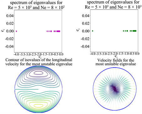
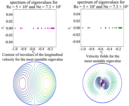
5.3. Axisymmetric Disturbance (n = 0, k₀ ≠ 0)

For this case, depends on space variables r and z and on time variable t. The eigenvalues found are certainly complex but have a common characteristic: their real parts are all negative. What also testifies to the stability of this flow although the term of inertia is not null.

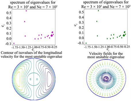
5.4. Three-Dimensional Disturbance (n ≠ 0, k₀ ≠ 0)

For the latter case, the disturbances depend not only on time but also on all the spatial variables. It is noted that as for the axisymmetric case, the eigenvalues are imaginary but each of them has a negative real part. Therefore, this flow is temporally stable. We also note that for the four cases studied above, when the Reynolds number Re is fixed, the variation of the dimensionless number Ne has no effect on the flow.

6. Conclusion

It has also been established that the linear flow of such a fluid is theoretically stable in the absence of a magnetic field. The flow of a Newtonian and non-conductive fluid subjected to a magnetic field is linearly stable. It is as if the magnetic field applied to the device introduces small disturbances to the flow. On the other hand, the intensification of the magnetic effects has no effect on the flow. Indeed, the volumetric magnetic force derives from a gradient; it is canceled gift by projection on the functions test which is functions with null divergence.

Acknowledgements

I thank my parents who sent and kept me in school. M. Mbow is the professor who introduced me to research, I will always grateful to him. To M. Sow, also, I say big thank you. He was my thesis director there. He is very available and is very concerned about the success of his students.

Appendix Code

The algorithm QZ makes possible to determine the eigenvalues and optionally the eigenvectors of the problem with generalized eigenvalues $Av=B\chi v$. The idea is to transform the matrices A and B into similar upper triangular matrices. If A and B are respectively upper Hessenberg and triangular matrices. We call

the QZ decomposition of pair $\left(A,B\right)$, the double factorization $\{\begin{array}{l}QA=R\\ \left(QB\right)Z=T\end{array}$ with Q unitary matrix, Z upper Hessenberg, R and T upper triangular. We will note later on $\{\begin{array}{l}QAZ=\tilde{A}\\ QBZ=\tilde{B}\end{array}$ we can construct a unitary decomposing matrix A, as

a product of n − 1 matrices of elementary rotation: $Q=Q^{\left(n-1\right)}\cdots Q^{\left(2\right)}{Q}^{\left(1\right)}$ where each $Q^{\left(i\right)}$ is a complex rotation matrix. $Q^{\left(i\right)}$ modifies the first and second lines of B possibly creating a non-zero element in position $\left(2,1\right)$ which will have to be cancelled by a complex rotation matrix $Z_1$ modifying only the first and the second column of $Q^{\left(1\right)}B$. Note $B^{\left(1\right)}=B$ and $B^{\left(2\right)}=Q^{\left(1\right)}{B}^{\left(1\right)}{Z}^{\left(1\right)}$. $B^{\left(2\right)}$ is triangular superior.

Let $B^{\left(k\right)}$ be upper triangular, let $Q^{\left(k\right)}$ be the rotation matrix modifying only the k^th and (k + 1)^th columns of $B^{\left(k\right)}$ possibly creating a non-zero element in position $\left(k+1,k\right)$ which will have to be cancelled by a matrix rotation $Z^{\left(k\right)}$ only modifying the k^th and (k + 1)^th columns of $Q^{\left(k\right)}{B}^{\left(k\right)}$. Let’s say $B^{\left(k+1\right)}$ is upper triangular, the process stops for k = n − 1 and we can write $\tilde{B}=QBZ=B^{\left(n\right)}$, $Z=Z^{\left(1\right)}\times Z^{\left(2\right)}\times \cdots \times Z^{\left(n-1\right)}$.

If B is invertible, it is obvious that Q realizes a unitary and triangular decomposition of $A{B}^{-1}$ and $Z^{\ast }$ a unitary decomposition of $B^{-1}A$, in fact:

$Z^{\ast }{B}^{-1}A=Z^{\ast }{B}^{-1}{Q}^{\ast }QA=\tilde{B}QA$

$\tilde{B}$ and QA are upper triangular. We obtain the eigenvalues by calculating the ratios of diagonal elements of QA and B.

Nomenclature

Greek letters

α: complex argument

θ: azimuthal coordinate

μ₀: electrical permeability in vacuum

ν: kinematic viscosity of the fluid

ρ: density of the fluid

η: dynamic viscosity of the fluid

ϕ: basic function

χ: electrical susceptibility

ψ: test function

Latin letters

$A$ : potential vector

$A_i$ : component of potential vector in the direction i

$B$ : magnetic field

$B_i$ : component of the magnetic field in the direction i

$C_i$ : imaginary part of eigenvalue

$C_r$ : real part of the eigenvalue

f: density force

$I_0$ : modified Bessel function of the first kind of order 0

$I_1$ : modified Bessel function of the first kind of order 1

$j$ : current density vector

$j_0$ : maximum value of current density

$l$ : axial mode

$k=k_0$ : axial wave number

$K_0$ : modified Bessel function of the second kind of order 0

$K_1$ : modified Bessel function of the second kind of order 1

n: azimuthal mode

Ne: new dimensionless number

p: pressure

r: radial coordinate

R: radius of the cylinder

Re: Reynold’s number

t: time variable

$u=u_b$ : fluid velocity not subjected to a magnetic field

$u_m$ : fluid velocity subjected to a magnetic field

$u_0$ : maximum steady state fluid velocity

$u^{\prime }$ : disturbance velocity field

z: axial coordinate

Conflicts of Interest

The authors declare no conflicts of interest regarding the publication of this paper.

References

[1]	Matsuzaki, A. and Nagakura, S. (1976) Magnetic Quenching of Fluorescence Observed with Carbon Disulfide and Glyoxal. Journal of Luminescence, 12-13, 787-791. https://doi.org/10.1016/0022-2313(76)90177-0
[2]	Kakeshita, T., et al. (1985) Composition Dependence of Magnetic Field-Induced Martensitic Transformations in Fe-Ni Alloys. Acta Metallurgica, 33, 1381-1389. https://doi.org/10.1016/0001-6160(85)90039-2
[3]	Aogaki, R., Fueki, K. and Mukaibo, T. (1975) Application of Magnetohydrodynamic Effect to the Analysis of Electrochemical Reactions. 2. Diffusion Process in MHD Forced Flow of Electrolyte Solution. Denki Kagaku, 43, 509-514. https://doi.org/10.5796/kogyobutsurikagaku.43.509
[4]	Torbet, J., Freyssinet, J.-M. and Hudry-Clergeon, G. (1981) Oriented Fibrin Gels Formed by Polymerization in Strong Magnetic Fields. Nature, 289, 91. https://doi.org/10.1038/289091a0
[5]	Meseguer, A. and Trefethen, L.N. (2003) Linearized Pipe Flow to Reynolds Number 107. Journal of Computational Physics, 186, 178-197. https://doi.org/10.1016/S0021-9991(03)00029-9
[6]	Zikanov, O.Yu. (1996) On the Instability of Pipe Poiseuille Flow. Physics of Fluids, 8, 2923. https://doi.org/10.1063/1.869071
[7]	Bergstrom, L. (1997) Optimal Growth of Small Disturbances in Pipe Poiseuille Flow. Physics of Fluids, 9, 1043.
[8]	Leonard, A. and Wray, A. (1982) A New Numerical Method for the Simulation of Three-Dimensional Flow in a Pipe. In: Krause, E., Ed., Proceedings of the 8th International Conference on Numerical Methods in Fluid Dynamics on Numerical Methods in Fluid Dynamics, Springer, Berlin, 335-342. https://doi.org/10.1007/3-540-11948-5_40
[9]	Schmid, P.J. and Henningson, D.S. (1994) Optimal Energy Grothin Hagen-Poiseuille Flow. Journal of Fluid Mechanics, 277, 197. https://doi.org/10.1017/S0022112094002739
[10]	Trefethen, A.E., Trefethen, L.N. and Schmid, P.J. (1999) Spectra and Pseudospectra for Pipe Poiseuille Flow. Computer Methods in Applied Mechanics and Engineering, 175, 413-420. https://doi.org/10.1016/S0045-7825(98)00364-8
[11]	Matsuzaki, A. and Nagakura, S. (1976) Magnetic Quenching of Fluorescence Observed with Carbon Disulfide and Glyoxal. Journal of Luminescence, 12-13, 787-791. https://doi.org/10.1016/0022-2313(76)90177-0
[12]	Kakeshita, T., et al. (1985) Composition Dependence of Magnetic Field-Induced Martensitic Transformations in Fe-Ni Alloys. Acta Metallurgica, 33, 1381-1389. https://doi.org/10.1016/0001-6160(85)90039-2
[13]	Aogaki, R., Fueki, K. and Mukaibo, T. (1975) Application of Magnetohydrodynamic Effect to the Analysis of Electrochemical Reactions. 2. Diffusion Process in MHD Forced Flow of Electrolyte Solution. Denki Kagaku, 43, 509-514. https://doi.org/10.5796/kogyobutsurikagaku.43.509
[14]	Torbet, J., Freyssinet, J.-M. and Hudry-Clergeon, G. (1981) Oriented Fibrin Gels Formed by Polymerization in Strong Magnetic Fields. Nature, 289, 91. https://doi.org/10.1038/289091a0
[15]	Meseguer, A. and Trefethen, L.N. (2003) Linearized Pipe Flow to Reynolds Number 107. Journal of Computational Physics, 186, 178-197. https://doi.org/10.1016/S0021-9991(03)00029-9
[16]	Zikanov, O.Yu. (1996) On the Instability of Pipe Poiseuille Flow. Physics of Fluids, 8, 2923. https://doi.org/10.1063/1.869071
[17]	Bergstrom, L. (1997) Optimal Growth of Small Disturbances in Pipe Poiseuille Flow. Physics of Fluids, 9, 1043.
[18]	Leonard, A. and Wray, A. (1982) A New Numerical Method for the Simulation of Three-Dimensional Flow in a Pipe. In: Krause, E., Ed., Proceedings of the 8th International Conference on Numerical Methods in Fluid Dynamics on Numerical Methods in Fluid Dynamics, Springer, Berlin, 335-342. https://doi.org/10.1007/3-540-11948-5_40
[19]	Schmid, P.J. and Henningson, D.S. (1994) Optimal Energy Grothin Hagen-Poiseuille Flow. Journal of Fluid Mechanics, 277, 197. https://doi.org/10.1017/S0022112094002739
[20]	Trefethen, A.E., Trefethen, L.N. and Schmid, P.J. (1999) Spectra and Pseudospectra for Pipe Poiseuille Flow. Computer Methods in Applied Mechanics and Engineering, 175, 413-420. https://doi.org/10.1016/S0045-7825(98)00364-8