Confidence Regions with Nuisance Parameters

Jan Vrbik

Department of Mathematics and Statistics, Brock University, St. Catharines, Canada.

DOI: 10.4236/ojs.2022.125039                

Abstract

Consider a distribution with several parameters whose exact values are unknown and need to be estimated using the maximum-likelihood technique. Under a regular case of estimation, it is fairly routine to construct a confidence region for all such parameters, based on the natural logarithm of the corresponding likelihood function. In this article, we investigate the case of doing this for only some of these parameters, assuming that the remaining (so called nuisance) parameters are of no interest to us. This is to be done at a chosen level of confidence, maintaining the usual accuracy of this procedure (resulting in about 1% error for samples of size , and further decreasing with 1/n). We provide a general solution to this problem, demonstrating it by many explicit examples.

Keywords

Confidence Regions, Maximum Likelihood, Nuisance Parameters, Asymptotic Distribution

1. Introduction

There is a basic technique (expounded in detail by M. S. Bartlett—see [1] [2] and [3] —nicely summarized in [4]) for constructing confidence regions (intervals) for parameters of a specific distribution (assuming a regular case, meaning the distribution’s support is not a function of any of the distribution’s parameters) which rests on the fact that

$2\ln \mathcal{L}\left(X\mathrm{<mo>\; ;\; </mo>}\hat{\theta }\right)-2\ln \mathcal{L}\left(X\mathrm{<mo>\; ;\; </mo>}{\theta }_0\right)$ (1)

has approximately the chi-square distribution with K degrees of freedom (K is the number of parameters to be estimated), where

$\ln \mathcal{L}\left(X\mathrm{<mo>\; ;\; </mo>}\theta \right)\mathrm{<mo>\; :\; </mo>}={\displaystyle \underset{i=1}{\overset{n}{\sum }}}\ln f\left(x_i\mathrm{<mo>\; ;\; </mo>}\theta \right)$ (2)

$X$ is the set of n observations, individually denoted $x_i$ (allowing for a possibility of a multivariate distribution), $f\left(x\mathrm{<mo>\; ;\; </mo>}\theta \right)$ denotes the corresponding probability density function, $\hat{\theta }$ is the vector of the resulting maximum-likelihood (ML) estimators of the parameters, and ${\theta }_0$ represents their true (even though unknown) values.

The proof rests on expanding the LHS of following K-component equation

${\displaystyle \underset{i=1}{\overset{n}{\sum }}}\frac{\partial \ln f\left(x_i\mathrm{<mo>\; ;\; </mo>}\theta \right)}{\partial \theta }=0$ (3)

with respect to $\theta$ at ${\theta }_0$ to a linear (in $\theta -{\theta }_0$ ) accuracy, making the answer equal to $0$ and solving for $\theta$, thereby getting

$\hat{\theta }-{\theta }_0\simeq {\mathbb{M}}^{-1}Y$ (4)

where

$Y\mathrm{<mo>\; :\; </mo>}=\frac{1}{n}{\displaystyle \underset{i=1}{\overset{n}{\sum }}}{\frac{\partial \ln f\left(x_i\mathrm{<mo>\; ;\; </mo>}\theta \right)}{\partial \theta }|}_{\theta ={\theta }_0}$ (5)

and

$\mathbb{M}\mathrm{<mo>\; :\; </mo>}=-\mathbb{E}\left({\frac{{\partial }^2\ln f\left(X\mathrm{<mo>\; ;\; </mo>}\theta \right)}{\partial {\theta }^2}|}_{\theta ={\theta }_0}\right)\equiv \mathbb{E}\left({\frac{\partial \ln f\left(X\mathrm{<mo>\; ;\; </mo>}\theta \right)}{\partial \theta }\circ \frac{\partial \ln f\left(X\mathrm{<mo>\; ;\; </mo>}\theta \right)}{\partial \theta }|}_{\theta ={\theta }_0}\right)$ (6)

Note that $Y$ is a K-component vector, while $\mathbb{M}$ represents a symmetric, positive-definite K by K matrix (the small circle stands for a direct product of two vectors).

Similarly expanding (1) and utilizing (4) we get

$2nY\left(\hat{\theta }-{\theta }_0\right)-n{\left(\hat{\theta }-{\theta }_0\right)}^{\text{T}}\mathbb{M}\left(\hat{\theta }-{\theta }_0\right)+\cdots =\sqrt{n}{Y}^{\text{T}}{\mathbb{M}}^{-1}Y\sqrt{n}$ (7)

where $Y\sqrt{n}$ has (by Central Limit Theorem), approximately, a K-variate Normal distribution with the mean of $0$ and the variance-covariance matrix of $\mathbb{M}$ ; this implies that (7) has, to the same level of approximation, the ${\chi }_K^2$ distribution (since the components of ${\mathbb{M}}^{-1/2}Y\sqrt{n}$ are then asymptotically independent, each having the mean of 0 and the variance of 1).

From all this, it then follows that an approximate confidence region is found by first finding the maximum likelihood estimators $\hat{\theta }$, then making (1) equal to a critical ${\chi }_K^2$ value and solving (usually, only graphically) for ${\theta }_0$.

We demonstrate this by generating a random independent sample of 200 observations from a Negative Binomial distribution (with parameters $\alpha$ and p) and constructing the corresponding 90% confidence region for the two parameters; a simple, self-explanatory Mathematica code to do exactly that looks like this:

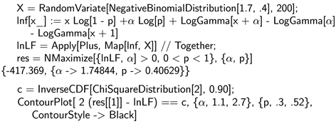
The resulting confidence region is displaced in Figure 1.

Similarly, to test a null hypothesis which claims specific values for the K parameters, we evaluate (1) with ${\theta }_0$ being the hypothesized (rather than the true) values, and check the result against the critical value of ${\chi }_K^2$ ; something this article will not elaborate on any further.

2. Partial Confidence Regions

The aim of this article is to show how to construct a confidence region (called partial) for only some parameters of distribution, even though all of its parameters are unknown and need to be estimated by the maximum-likelihood technique.

We should mention that there is some existing literature on using partial likelihood functions (LF), for example [5], but its goals and results bear little resemblance to ours. Similarly, articles on marginal LF (for example [6]) and conditional LF deal with only rather specialized issues while our approach is fully general; the only shared feature is the occasional use of identical terminology.

Figure 1. 90% confidence region for α and p.

Extending the technique delineated in our Introduction, we now need to find an approximate distribution of

$2\ln \mathcal{L}\left(X\mathrm{<mo>\; ;\; </mo>}\hat{\theta }\right)-2\ln \mathcal{L}\left(X\mathrm{<mo>\; ;\; </mo>}{\hat{\Theta }}_0\right)$ (8)

where only some components of ${\hat{\Theta }}_0$ are equal to the true values of the corresponding (we call them pivotal) parameters, while the rest (the nuisance parameters; a term introduced by [7] and further explored by [8]) are set to their $\hat{\theta }$ values. Knowing this distribution will then enable us to construct confidence regions (or test hypotheses) for the pivotal parameters only while ignoring the estimates of the nuisance parameters.

Since we already have a good approximation to (1), namely (7), or equivalently

$\sqrt{n}{\left(\hat{\theta }-{\theta }_0\right)}^{\text{T}}\mathbb{M}\left(\hat{\theta }-{\theta }_0\right)\sqrt{n}$ (9)

we now need a similar approximation for

$2\ln L\left(X\mathrm{<mo>\; ;\; </mo>}{\hat{\Theta }}_0\right)-2\ln L\left(X\mathrm{<mo>\; ;\; </mo>}{\theta }_0\right)$ (10)

and then, for the corresponding difference. To approximate (10), we go back to the LHS of (7) and replace $\hat{\theta }-{\theta }_0$ by ${\hat{\Theta }}_0-{\theta }_0$ (i.e. keeping the nuisance components of $\hat{\theta }-{\theta }_0$ and setting the pivotal components to 0) while $Y=\mathbb{M}\left(\hat{\theta }-{\theta }_0\right)$, computed from (4), remains unchanged. This results in

$\begin{array}{l}2n{\left(\hat{\theta }-{\theta }_0\right)}^{\text{T}}\mathbb{M}\left({\hat{\Theta }}_0-{\theta }_0\right)-n{\left({\hat{\Theta }}_0-{\theta }_0\right)}^{\text{T}}\mathbb{M}\left({\hat{\Theta }}_0-{\theta }_0\right)\\ \mathrm{<mo>\; :\; </mo>}=n{\left(\hat{\theta }-{\theta }_0\right)}^{\text{T}}{\mathbb{M}}_0\left(\hat{\theta }-{\theta }_0\right)\end{array}$ (11)

where ${\mathbb{M}}_0$ is the original $\mathbb{M}$ matrix with all pivotal-by-pivotal elements set to 0 (a notation to be used with other matrices as well).

This can be shown by rearranging the parameters to start with the pivotal and be followed by the nuisance ones, and visualizing the corresponding 2 by 2 block structure of the symmetric matrix $\mathbb{M}$. In such representation, the previous equation reads

$n{\left(\hat{\theta }-{\theta }_0\right)}^{\text{T}}\left[\begin{array}{cc}\mathbb{O}& ■\\ \mathbb{O}& ■\end{array}\right]\left(\hat{\theta }-{\theta }_0\right)+n{\left(\hat{\theta }-{\theta }_0\right)}^{\text{T}}\left[\begin{array}{cc}\mathbb{O}& \mathbb{O}\\ ■& ■\end{array}\right]\left(\hat{\theta }-{\theta }_0\right)$

$-n{\left(\hat{\theta }-{\theta }_0\right)}^{\text{T}}\left[\begin{array}{cc}\mathbb{O}& \mathbb{O}\\ \mathbb{O}& ■\end{array}\right]\left(\hat{\theta }-{\theta }_0\right)=n{\left(\hat{\theta }-{\theta }_0\right)}^{\text{T}}\left[\begin{array}{cc}\mathbb{O}& ■\\ ■& ■\end{array}\right]\left(\hat{\theta }-{\theta }_0\right)$

where a full square $■$ indicates keeping the original block of the $\mathbb{M}$ matrix, while each $\mathbb{O}$ represents a zero sub-matrix of the corresponding dimensions.

Subtracting (11) from (9) then yields the desired approximation to (8), namely

$\sqrt{n}{\left(\hat{\theta }-{\theta }_0\right)}^{\text{T}}\left(\mathbb{M}-{\mathbb{M}}_0\right)\left(\hat{\theta }-{\theta }_0\right)\sqrt{n}$ (12)

Introducing $U=\left(\hat{\theta }-{\theta }_0\right)\sqrt{n}$, which we know from our Introduction to be approximately K-variate Normal, having zero means and the variance-covariance matrix of ${\mathbb{M}}^{-1}$, we can now find the moment generating function (MGF) of (12) by

$\begin{array}{l}\frac{{\displaystyle \int \cdots }{\displaystyle {\int }_{-\infty }^{\infty }\exp }\left(-\frac{u^{\text{T}}\mathbb{M}u}{2}+t{u}^{\text{T}}\left(\mathbb{M}-{\mathbb{M}}_0\right)u\right)\text{d}u}{{\left(2\pi \right)}^{K/2}\sqrt{\det \left({\mathbb{M}}^{-1}\right)}}\\ =\sqrt{\frac{1}{\det \left(\mathbb{I}-2t\mathbb{I}+2t{\mathbb{M}}_0{\mathbb{M}}^{-1}\right)}}=\sqrt{\frac{1}{\det \left(\mathbb{I}-2t\mathbb{I}+2t\mathbb{M}{\left({\mathbb{M}}^{-1}\right)}_0\right)}}\end{array}$ (13)

where $\mathbb{I}$ is the K by K identity matrix. The last equality follows from the fact that

${\mathbb{M}}_0{\mathbb{M}}^{-1}=\left[\begin{array}{cc}{\mathbb{M}}_{p,i}{\left({\mathbb{M}}^{-1}\right)}_{i,p}& \cdots \\ \mathbb{O}& \mathbb{I}\end{array}\right]=\left[\begin{array}{cc}\mathbb{I}-{\mathbb{M}}_{p,p}{\left({\mathbb{M}}^{-1}\right)}_{p,p}& \cdots \\ \mathbb{O}& \mathbb{I}\end{array}\right]$ (14)

and

$\mathbb{M}{\left({\mathbb{M}}^{-1}\right)}_0=\left[\begin{array}{cc}{\mathbb{M}}_{p,i}{\left({\mathbb{M}}^{-1}\right)}_{i,p}& \mathbb{O}\\ \cdots & \mathbb{I}\end{array}\right]$ (15)

make the same contribution to the determinant in (13), where $\mathbb{I}$ is now the L by L identity matrix (L being the number of pivotal parameters). In (14), we also use the fact that

${\mathbb{M}}_{p,i}{\left({\mathbb{M}}^{-1}\right)}_{i,p}+{\mathbb{M}}_{p,p}{\left({\mathbb{M}}^{-1}\right)}_{p,p}=\mathbb{I}$ (16)

where the $p$ and $i$ subscripts refer to the corresponding pivotal and/or nuisance block of the matrix.

It is easy to see that the result of (13) does not change after replacing $\mathbb{M}$ (the variance-covariance matrix of $\sqrt{n}Y$ ) by the corresponding correlation matrix $ℂ={\mathbb{D}}^{-1/2}\mathbb{M}{\mathbb{D}}^{-1/2}$, where $\mathbb{D}$ is the main-diagonal matrix of the corresponding variances, and correspondingly replacing ${\mathbb{M}}_0$ by ${ℂ}_0={\left({\mathbb{D}}^{-1/2}\mathbb{M}{\mathbb{D}}^{-1/2}\right)}_0={\mathbb{D}}^{-1/2}{\mathbb{M}}_0{\mathbb{D}}^{-1/2}$ (recall that the 0 subscript indicates setting all pivotal-pivotal elements equal to 0), since clearly

$\det \left(\mathbb{I}-2t\mathbb{I}+2t{\mathbb{M}}_0{\mathbb{M}}^{-1}\right)=\det \left(\mathbb{I}-2t\mathbb{I}+2t{ℂ}_0{ℂ}^{-1}\right)$ (17)

Similarly, we can replace the asymptotic variance-covariance matrix of $\sqrt{n}\left(\hat{\theta }-{\theta }_0\right)$, namely ${\mathbb{M}}^{-1}$, by its correlation matrix $\widetilde{ℂ}={\tilde{\mathbb{D}}}^{-1/2}{\mathbb{M}}^{-1}{\tilde{\mathbb{D}}}^{-1/2}$ and ${\mathbb{M}}_0$ by ${\left({\widetilde{ℂ}}^{-1}\right)}_0={\tilde{\mathbb{D}}}^{1/2}{\mathbb{M}}_0{\tilde{\mathbb{D}}}^{1/2}$ without affecting the value of the determinant.

Summary

Based on (14), the MGF of (12) is given by

${\displaystyle \underset{\mathcal{l}=1}{\overset{L}{\prod }}\frac{1}{\sqrt{1-2t\cdot e_{\mathcal{l}}}}}$ (18)

where $e_1\mathrm{,}{e}_2\mathrm{,}\cdots ,e_L$ are the eigenvalues of ${\mathbb{M}}_{p,p}{\left({\mathbb{M}}^{-1}\right)}_{p,p}$ (note that $\mathbb{M}$ can be replaced by $ℂ$ or $\widetilde{ℂ}$, whichever is more convenient). The resulting PDF is then that of a convolution of the individual Gamma ( $\frac{1}{2}\mathrm{,2}{e}_{\mathcal{l}}$ ) distributions.

It is important to note that, when there are more pivotal than nuisance parameters (i.e. when $L>K-L$ ), the L by L matrix ${\mathbb{M}}_{p,i}{\left({\mathbb{M}}^{-1}\right)}_{i,p}$ in (16) is of rank $K-L$ only (this is now determined by the number of columns of ${\mathbb{M}}_{p,i}$ ), implying that $L-\left(K-L\right)=2L-K$ of its eigenvalues are equal to 0, and correspondingly simplifying the eigenvalues of ${\mathbb{M}}_{p,p}{\left({\mathbb{M}}^{-1}\right)}_{p,p}$ ( $2L-K$ of which will be equal to 1). Furthermore, the remaining eigenvalues of ${\mathbb{M}}_{p,i}{\left({\mathbb{M}}^{-1}\right)}_{i,p}$ are the same as those of ${\mathbb{M}}_{i,p}{\left({\mathbb{M}}^{-1}\right)}_{p,i}$ ; this is based on a general result stating that, when $\mathbb{A}$ is an n by m matrix while $\mathbb{B}$ is m by n, $\mathbb{A}\mathbb{B}$ and $\mathbb{B}\mathbb{A}$ will share all their non-zero eigenvalues, while the extra eigenvalues, if any, will be equal to 0.

This implies that, when $L>K-L$, we can replace the eigenvalues of ${\mathbb{M}}_{p,p}{\left({\mathbb{M}}^{-1}\right)}_{p,p}$ by the eigenvalues of ${\mathbb{M}}_{i,i}{\left({\mathbb{M}}^{-1}\right)}_{i,i}$ (a smaller matrix), knowing that each of the remaining $2L-K$ eigenvalues is equal to 1.

The final note: some steps of the resulting procedure for constructing partial confidence regions may be carried out analytically, while the rest require a numerical approach. This can be observed in our subsequent examples: some avoid explicit formulas entirely, performing each step numerically (always an available option), while our last example is almost completely analytical, to facilitate investigation of the technique’s accuracy.

3. Multivariate Normal Distribution

The most important multi-parameter distribution is the Normal distribution of several (say n) random variables $X_1\mathrm{,}{X}_2\mathrm{,}\cdots ,X_n$, collectively denoted $X$. It is fully specified by the following parameters: n individual means (collectively denoted $\mu$ ), n standard deviations $\sigma$, and $\left(\begin{array}{c}n\\ 2\end{array}\right)$ correlation coefficients ${\rho }_{ij}$ ( $1\le i<j\le n$ ) usually collected in a symmetric matrix $ℝ$ (each ${\rho }_{ij}$ will

appear twice, on both sides of the main diagonal, whose elements are all equal to 1). This section is a review of basic formulas relating to ML estimation of these parameters.

The natural logarithm of the corresponding PDF (aka likelihood function) is given by

$-\frac{{\left(x-\mu \right)}^{\text{T}}{\mathbb{S}}^{-1}{ℝ}^{-1}{\mathbb{S}}^{-1}\left(x-\mu \right)}{2}-\frac{1}{2}\ln \det ℝ-\ln \det \mathbb{S}-\frac{n}{2}\ln \left(2\pi \right)$ (19)

where $\mathbb{S}$ is a main-diagonal matrix of the n values of $\sigma$. Note that ${\mathbb{S}}^{-1}\left(x-\mu \right)$, explicitly expanded, yields the following vector $\langle \frac{x_1-{\mu }_1}{{\sigma }_1}\mathrm{,}\frac{x_2-{\mu }_2}{{\sigma }_2}\mathrm{,}\cdots ,\frac{x_n-{\mu }_n}{{\sigma }_n}\rangle$.

To find the corresponding $\mathbb{M}$ matrix, we use the following well-known formulas

$\frac{\text{d}{ℝ}^{-1}}{\text{d}{\rho }_{kl}}\mathrm{<mo>\; =\; </mo>}-{ℝ}^{-1}\frac{\text{d}ℝ}{\text{d}{\rho }_{kl}}{ℝ}^{-1}$ (20)

$\frac{\text{d}\ln \det ℝ}{\text{d}{\rho }_{kl}}=\text{Tr}\left(\frac{\text{d}ℝ}{\text{d}{\rho }_{kl}}{ℝ}^{-1}\right)$ (21)

where Tr indicates taking the matrix’ trace. Note that all but two elements of

$\frac{\text{d}ℝ}{\text{d}{\rho }_{kl}}\mathrm{<mo>\; :\; </mo>}={ℍ}^{\left[kl\right]}=v^{\left[k\right]}\circ v^{\left[l\right]}+v^{\left[l\right]}\circ v^{\left[k\right]}$ (22)

are equal to 0 (the remaining two elements are equal to 1), where $v^{\left[k\right]}$ stands for a vector of $n-1$ zeros with only its k^th component equal to 1.

Differentiating (19) twice with respect to $\mu$ and changing the sign yields

${\mathbb{S}}^{-1}{ℝ}^{-1}{\mathbb{S}}^{-1}$ (23)

which represents the $\mu$ by $\mu$ block of $\mathbb{M}$, while the $\mu$ by $\sigma$ and $\mu$ by ${\rho }_{ij}$ blocks are both zero sub-matrices, since $\mathbb{E}\left(x-\mu \right)=0$ —that goes for the $\sigma$ by $\mu$ and ${\rho }_{ij}$ by $\mu$ blocks as well.

To find the $\sigma$ by $\sigma$ block, we first differentiate (19) with respect to ${\sigma }_i$ and then with respect to ${\sigma }_j$ (assuming $i\ne j$ ), getting

$-\frac{{\left(x-\mu \right)}_i{\left({ℝ}^{-1}\right)}_{ij}{\left(x-\mu \right)}_j+{\left(x-\mu \right)}_j{\left({ℝ}^{-1}\right)}_{ij}{\left(x-\mu \right)}_i}{2{\sigma }_i^2{\sigma }_j^2}$ (24)

Reversing the sign and taking the expected value yields the following expression for the off-diagonal elements of the $\sigma$ by $\sigma$ block

$\frac{{ℝ}_{ij}{\left({ℝ}^{-1}\right)}_{ij}}{{\sigma }_i{\sigma }_j}$ (25)

since $\mathbb{E}\left(\left(x_i-{\mu }_i\right)\left(x_j-{\mu }_j\right)\right)={\sigma }_i{\sigma }_j{ℝ}_{ij}$.

When differentiating with respect of ${\sigma }_i$ twice, the corresponding second derivative is

$\begin{array}{l}-{\displaystyle \underset{j=1}{\overset{n}{\sum }}}\frac{{\left(x-\mu \right)}_i{\left({ℝ}^{-1}\right)}_{ij}{\left(x-\mu \right)}_j+{\left(x-\mu \right)}_j{\left({ℝ}^{-1}\right)}_{ij}{\left(x-\mu \right)}_i}{{\sigma }_i^3{\sigma }_j}\\ -\frac{{\left(x-\mu \right)}_i{\left({ℝ}^{-1}\right)}_{ii}{\left(x-\mu \right)}_i}{{\sigma }_i^4}+\frac{1}{{\sigma }_i^2}\end{array}$ (26)

Reversing the sign and taking the expected value then yields

$2{\displaystyle \underset{j=1}{\overset{n}{\sum }}}\frac{{\left({ℝ}^{-1}\right)}_{ij}{ℝ}_{ji}}{{\sigma }_i^2}+\frac{{ℝ}_{ii}{\left({ℝ}^{-1}\right)}_{ii}}{{\sigma }_i^2}-\frac{1}{{\sigma }_i^2}=\frac{{ℝ}_{ii}{\left({ℝ}^{-1}\right)}_{ii}}{{\sigma }_i^2}+\frac{1}{{\sigma }_i^2}$ (27)

for the main-diagonal elements of the $\sigma$ by $\sigma$ block (note that ${\displaystyle {\sum }_{j=1}^n}{\left({ℝ}^{-1}\right)}_{ij}{ℝ}_{ji}={\mathbb{I}}_{ii}=1$ ).

This means that

$\frac{{ℝ}_{ij}{\left({ℝ}^{-1}\right)}_{ij}+{\mathbb{I}}_{ij}}{{\sigma }_i{\sigma }_j}$ (28)

is the resulting expression for both the diagonal and off-diagonal elements of the $\sigma$ by $\sigma$ block.

To find the ${\rho }_{kl}$ - ${\rho }_{mp}$ element of the $\mathbb{M}$ matrix, we first need the corresponding second derivative of (19), namely

$-\frac{2{\left(x-\mu \right)}^{\text{T}}{\mathbb{S}}^{-1}{ℝ}^{-1}{ℍ}^{\left[kl\right]}{ℝ}^{-1}{ℍ}^{\left[mp\right]}{ℝ}^{-1}{\mathbb{S}}^{-1}\left(x-\mu \right)}{2}+\frac{1}{2}\text{Tr}\left({ℍ}^{\left[kl\right]}{ℝ}^{-1}{ℍ}^{\left[mp\right]}{ℝ}^{-1}\right)$ (29)

Reversing the sign and taking the expected value results in

$\frac{1}{2}\text{Tr}\left({ℍ}^{\left[kl\right]}{ℝ}^{-1}{ℍ}^{\left[mp\right]}{ℝ}^{-1}\right)={\left({ℝ}^{-1}\right)}_{km}{\left({ℝ}^{-1}\right)}_{lp}+{\left({ℝ}^{-1}\right)}_{kp}{\left({ℝ}^{-1}\right)}_{lm}$ (30)

Finally, to get the ${\sigma }_i$ - ${\rho }_{kl}$ element of $\mathbb{M}$, the corresponding differentiation of (19) yields

$-\frac{{\left(x-\mu \right)}_i{\mathbb{S}}^{-1}{ℝ}^{-1}{ℍ}^{\left[kl\right]}{ℝ}^{-1}{\mathbb{S}}^{-1}\left(x-\mu \right)+{\left(x-\mu \right)}^{\text{T}}{\mathbb{S}}^{-1}{ℝ}^{-1}{ℍ}^{\left[kl\right]}{ℝ}^{-1}{\mathbb{S}}^{-1}{\left(x-\mu \right)}_i}{2{\sigma }_i}$ (31)

which, after changing the sign and taking the expected value, results in

${\displaystyle \underset{j=1}{\overset{n}{\sum }}}\frac{{ℝ}_{ij}{\left({ℝ}^{-1}{ℍ}^{\left[kl\right]}{ℝ}^{-1}\right)}_{ji}}{{\sigma }_i}=\frac{{\left({ℍ}^{\left[kl\right]}{ℝ}^{-1}\right)}_{ii}}{{\sigma }_i}=\frac{{\left({ℝ}^{-1}\right)}_{ik}{\mathbb{I}}_{il}+{\left({ℝ}^{-1}\right)}_{il}{\mathbb{I}}_{ik}}{{\sigma }_i}$ (32)

having a non-zero value only when $i=k$ or $i=l$.

4. Case of Asymptotic Independence

This section discusses the situation in which all elements of the pivotal-nuisance and (consequently) nuisance-pivotal blocks of $\mathbb{M}$ (and, correspondingly, of ${\mathbb{M}}_0$ and ${\mathbb{M}}^{-1}$ ) are equal to 0. In that case, ${\mathbb{M}}_0{\mathbb{M}}^{-1}$ has the following simple form: its nuisance-nuisance block is the identity matrix, the remaining three blocks are all zero sub-matrices (implying that $\mathbb{I}-{\mathbb{M}}_0{\mathbb{M}}^{-1}$ of (13) has an identity matrix in the pivotal-pivotal block, and zero sub-matrices elsewhere). The resulting MGF of (8) thus equals to ${\left(1-2t\right)}^{-L}$, where L is the number of pivotal parameters, which means that the asymptotic distribution of (8) is ${\chi }_L^2$, making a construction of the corresponding partial confidence region fairly routine.

Let us add that such asymptotic independence is not uncommon; for example, when a symmetric (with respect to its mean) distribution has a location and scale parameters only, the corresponding ML estimators are then always asymptotically independent.

To see why, note that, in this case, the PDF of the sampled distribution can be expressed as

$f\left(x\right)=\frac{1}{\sigma }\cdot f_0\left(\frac{x-\mu }{\sigma }\right)$ (33)

where $\mu$ and $\sigma$ are the location and scale parameters respectively, and $f_0\left(y\right)$ is a parameter-free PDF, symmetric with respect to 0. The off-diagonal element of $\mathbb{M}$ is then proportional to

${\displaystyle {\int }_{-\infty }^{\infty }}{f^{\prime }}_0\left(y\right)\cdot \frac{y\cdot {f^{\prime }}_0\left(y\right)+f_0\left(y\right)}{f_0\left(y\right)}\text{d}y$ (34)

due to (6); the integrand is clearly an anti-symmetric (odd) function of y, resulting in a zero integral. This enables us to find a partial confidence interval for either $\mu$ of for $\sigma$ (while ignoring the other parameter) by using the ${\chi }_1^2$ distribution for (8).

Similarly, in the case of a bivariate Normal distribution, the ML estimators of the two means on one hand, and of the two standard deviations and the correlation coefficient on the other, form two such mutually independent sets as well; this is clear from what we learned in the previous section but, due to the importance of this example, let us be more explicit and quote the well-known asymptotic correlation matrix of $\sqrt{n}\left(\hat{\theta }-{\theta }_0\right)$, namely

$\widetilde{ℂ}=\left[\begin{array}{ccccc}1& \rho & 0& 0& 0\\ \rho & 1& 0& 0& 0\\ 0& 0& 1& {\rho }^2& -\frac{\rho }{\sqrt{2}}\\ 0& 0& {\rho }^2& 1& -\frac{\rho }{\sqrt{2}}\\ 0& 0& -\frac{\rho }{\sqrt{2}}& -\frac{\rho }{\sqrt{2}}& 1\end{array}\right]$ (35)

where the five parameters (collectively denoted $\theta$ ) are the usual ${\mu }_1\mathrm{,}{\mu }_2\mathrm{,}{\sigma }_1\mathrm{,}{\sigma }_2$ and $\rho$ (in that order); the respective asymptotic variances are ${\sigma }_1^2/n\mathrm{,}{\sigma }_2^2/n\mathrm{,\; <mtext>\; \hspace{0.17em}\; </mtext>}{\sigma }_1^2/\left(2n\right)\mathrm{,\; <mtext>\; \hspace{0.17em}\; </mtext>}{\sigma }_2^2/\left(2n\right)$ and ${\left(1-{\rho }^2\right)}^2/n$.

Constructing a confidence region for either set of parameters is then quite simple (knowing that $\widetilde{ℂ}$ has the above block-diagonal structure is all we need, the individual elements are irrelevant) as the following Mathematica program demonstrates.

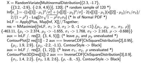
The program produces the output presented in Figure 2 and Figure 3; the first graph is the resulting partial 95% confidence region for ${\mu }_1$ and ${\mu }_2$, the second one is the 90% confidence region for ${\sigma }_1\mathrm{,}{\sigma }_2$ and $\rho$. This assumes that one is interested only in one or the other (not both)—if a confidence region for all five parameters is desired, one would use the basic procedure of our Introduction.

5. General Case

In general (and with no asymptotic independence to help) things get more complicated. We now go over all possible cases involving up to five parameters.

Figure 2. Confidence region for μ₁ and μ₂.

Figure 3. Confidence region for σ₁, σ₂ and ρ.

5.1. Two Parameters

In this situation, the only possibility is constructing a confidence interval for one of the two parameters, while ignoring the other. Since the $ℂ$ (or $\widetilde{ℂ}$ ) matrix will always have the following form

$ℂ=\left[\begin{array}{cc}1& \rho \\ \rho & 1\end{array}\right]$ (36)

we get

${ℂ}_{\mathrm{1,1}}{\left({ℂ}^{-1}\right)}_{\mathrm{1,1}}=\frac{1}{1-{\rho }^2}$ (37)

which implies that the distribution of (8) is that of a ${\chi }_1^2$ random variable, further divided by $1-{\rho }^2$. This means that, to construct a $1-\alpha$ confidence interval (CI) for the pivotal parameter, we make (8) equal to the corresponding critical value of ${\chi }_1^2$, also divided by $1-{\rho }^2$, substitute the ME estimate of the nuisance parameter, and solve for the pivotal one to get the two CI boundaries.

The following Mathematica program demonstrates the construction of a 90% confidence interval for the $\alpha$ parameter of the Gamma ( $\alpha \mathrm{,}\beta$ ) distribution.

Note that in this case $\rho =1/\sqrt{\alpha {\psi }_1}$, based on

$\mathbb{M}=\left[\begin{array}{cc}{\psi }_1& \frac{1}{\beta }\\ \frac{1}{\beta }& \frac{\alpha }{{\beta }^2}\end{array}\right]$ (38)

where ${\psi }_1$ is the second derivative of $\ln \Gamma \left(\alpha \right)$, called “PolyGamma[1, α]” by Mathematica; to evaluate it, we had to use the ML estimate of $\alpha$, instead of its true value. That is how we deal with this problem in general; this does not change the asymptotic distribution of (8).

5.2. Three Parameters

A three-parameter situation requires discussing two possibilities:

When constructing a CI for a single parameter (say ${\theta }_1$ ), (8) has again the ${\chi }_1^2\cdot {\left({ℂ}^{-1}\right)}_{\mathrm{1,1}}\equiv {\chi }_1^2\cdot {\left({\widetilde{ℂ}}^{-1}\right)}_{\mathrm{1,1}}$ distribution; this follows from ${ℂ}_{\mathrm{1,1}}{\left({ℂ}^{-1}\right)}_{\mathrm{1,1}}$ having only one element (its only eigenvalue), and from ${ℂ}_{\mathrm{1,1}}\equiv 1$. Note that this result (when interested in only one parameter) is true for any K.

When finding a confidence region for ${\theta }_2$ and ${\theta }_3$, the distribution of (8) is a convolution (i.e. an independent sum) of ${\chi }_1^2$ and another ${\chi }_1^2$, the latter multiplied $s\mathrm{<mo>\; :\; </mo>}={\left({ℂ}^{-1}\right)}_{\mathrm{1,1}}$ ; this is based on the arguments following (18). The corresponding PDF is

$\frac{1}{2\sqrt{s}}\exp \left(-\frac{s+1}{4s}\cdot y\right)I_0\left(\frac{s-1}{4s}\cdot y\right)$ (39)

where $I_0$ denotes the modified Bessel function of the first kind; note that using this PDF to find a critical value can be done only numerically (there is no analytic expression for the corresponding CDF, let alone for its inverse).

As an example, we assume sampling a distribution with the following PDF

$f\left(x\mathrm{<mo>\; ;\; </mo>}\alpha \mathrm{,}\beta \mathrm{,}\gamma \right)=\frac{\gamma \mathrm{<mtext>\; \hspace{0.17em}\; </mtext>}{x}^{\alpha -1}\exp \left(-{\left(\frac{x}{\beta }\right)}^{\gamma }\right)}{\Gamma \left(\frac{\alpha }{\gamma }\right)}\text{when}x>0$ (40)

(each of the three parameters must be positive) and constructing a 95% confidence region for $\beta$ and $\gamma$ only. Leaving out routine details, the expression for s turns out to be

$s=1+\frac{\alpha }{\gamma }+\frac{{\alpha }^2{\psi }_1-\left(\alpha +\gamma \right)\gamma }{{\gamma }^2+{\psi }_1\left({\gamma }^2-{\alpha }^2{\psi }_1\right)}$ (41)

where ${\psi }_1$ is the second derivative of $\ln \Gamma$, evaluated at $\frac{\alpha }{\gamma }$.

The following Mathematica code demonstrates the algorithm.

The confidence region for the $\beta$ and $\gamma$ thus produced is displayed in Figure 4.

Figure 4. Confidence region for β and γ.

5.3. Four Parameters

A CI for ${\theta }_1$ results in (8) having the ${\chi }_1^2\cdot {\left({ℂ}^{-1}\right)}_{\mathrm{1,1}}$ distribution, as discussed previously.

The complementary task of constructing a confidence region for ${\theta }_2\mathrm{,}{\theta }_3$ and ${\theta }_4$ then leads to a convolution of the previous distribution and that of ${\chi }_2^2$ (to account for the two extra eigenvalues of $\mathbb{I}-{ℂ}_{p,1}{\left({ℂ}^{-1}\right)}_{1,p}$, both equal to 1); this convolution has a PDF given by

$\frac{1}{2\sqrt{1-s}}\exp \left(-\frac{y}{2}\right)\text{erf}\left(\sqrt{\frac{\left(1-s\right)\cdot y}{2s}}\right)$ (42)

Finally, to build a confidence region for ${\theta }_1$ and ${\theta }_2$ requires using the following PDF for (8):

$\frac{\sqrt{t_1{t}_2}}{2}\exp \left(-\frac{t_1+t_2}{4}\cdot y\right)I_0\left(\frac{t_1-t_2}{4}\cdot y\right)$ (43)

where $t_1$ and $t_2$ are the two eigenvalues of ${\mathbb{M}}_{p,p}{\left({\mathbb{M}}^{-1}\right)}_{p,p}$ ; using $ℂ$ instead of $\mathbb{M}$ is still possible, but has no longer any advantage, since critical values of (42) and (43) can again be found only numerically.

To show how to use the last formula, we assume sampling a mixture of Exponential and Normal distributions (the four parameters are: the mean of the Exponential distribution, denoted b, and its weight in the mixturea, followed by the mean c and standard deviation d of the Normal distribution). Note that in this example we also bypass an analytic solution for elements of the $\mathbb{M}$ matrix—these can be easily computed by substituting values of the ML estimates for ${\theta }_0$ in (6), and only then computing, by numerical integration, the corresponding expected value. The following Mathematica program demonstrates the complete algorithm.

Producing the 90% confidence region displayed in Figure 5 for the mean (horizontal scale) and standard deviation (vertical scale) of the Normal-distribution part of the mixture.5.4. Five ParametersAs in all previous cases, a confidence interval for only one (say ${\theta }_1$ ) of the parameters requires using the ${\chi }_1^2$ distribution, further multiplied by $s\mathrm{<mo>\; :\; </mo>}={\left({ℂ}^{-1}\right)}_{\mathrm{1,1}}$.

Figure 5. Confidence region for c and d.

For the complementary task of building a (four-dimensional) confidence region for ${\theta }_2\mathrm{,}{\theta }_3\mathrm{,}{\theta }_4$ and ${\theta }_5$, the distribution of (8) becomes a convolution of ${\chi }_1^2\cdot s$ and ${\chi }_3^2$ ; the corresponding PDF is

$\frac{y}{4\sqrt{s}}\exp \left(-\frac{s+1}{4s}\cdot y\right)\left[I_0\left(\frac{s-1}{4s}\cdot y\right)+I_1\left(\frac{1-s}{4s}\cdot y\right)\right]$ (44)

A confidence region for ${\theta }_1$ and ${\theta }_2$ is found using the PDF of (43), found in the case of four parameters.

The PDF used for the three-dimensional confidence region of the true values of ${\theta }_3\mathrm{,}{\theta }_4$ and ${\theta }_5$ is then a convolution of the last PDF and that of an independent ${\chi }_1^2$ ; no explicit formula for the resulting PDF exists, but the following example demonstrates how to bypass this problem.

This time, we assume sampling a tri-variate Normal distribution having identical means (denoted $\mu$ ) and identical standard deviations (denoted $\sigma$ ). We now construct a three-dimensional confidence region for $\mu ,\sigma$ and ${\rho }_{12}$ (while ignoring ${\rho }_{13}$ and ${\rho }_{23}$ ), using the following Mathematica code.

The resulting confidence region is shown in Figure 6.

Figure 6. Confidence region for μ, σ and ρ₁₂.

6. Technique’s Accuracy

In this section, we go over a rather special example, allowing us to analytically find not only all ML estimators, but also an exact expression for (8). These are then used to build (still analytically) formulas for boundaries of a confidence interval for one of the parameters. Furthermore, the exact distribution of the estimator is also known, which gives us a unique opportunity to compute the error of our technique.

Let us now proceed with the actual example of constructing a confidence interval for the correlation coefficient of a bivariate Normal distribution, and computing its exact level of confidence (while ignoring the remaining four parameters).

Firstly, it is well known what the ML estimators of the two means ( ${\mu }_x$ and ${\mu }_y$ ), the two standard deviations ( ${\sigma }_x$ and ${\sigma }_y$ ), and the correlation coefficient $\rho$ are; we will denote them $\bar{X}\mathrm{,}\bar{Y}\mathrm{,}{S}_x\mathrm{,}{S}_y$ and r respectively. The likelihood function, once we replace all five parameters by their estimators, then reads

$\begin{array}{l}-\frac{1}{2\left(1-r^2\right)}{\displaystyle \underset{i=1}{\overset{n}{\sum }}}\left(\frac{{\left(X_i-\bar{X}\right)}^2}{S_x^2}+\frac{{\left(Y_i-\bar{Y}\right)}^2}{S_y^2}-2r\frac{\left(X_i-\bar{X}\right)\left(Y_i-\bar{Y}\right)}{S_x{S}_y}\right)\\ -\frac{n}{2}\ln \left(1-r^2\right)-n\ln S_x-n\ln S_y=-n-\frac{n}{2}\ln \left(1-r^2\right)-n\ln S_x-n\ln S_y\end{array}$ (45)

When similarly replacing the first four parameters only (keeping the exact value of $\rho$ ), the likelihood function becomes

$\begin{array}{l}-\frac{1}{2\left(1-{\rho }^2\right)}{\displaystyle \underset{i=1}{\overset{n}{\sum }}}\left(\frac{{\left(X_i-\bar{X}\right)}^2}{S_x^2}+\frac{{\left(Y_i-\bar{Y}\right)}^2}{S_y^2}-2\rho \frac{\left(X_i-\bar{X}\right)\left(Y_i-\bar{Y}\right)}{S_x{S}_y}\right)\\ -\frac{n}{2}\ln \left(1-{\rho }^2\right)-n\ln S_x-n\ln S_y=-n\frac{1-\rho \mathrm{<mtext>\; \hspace{0.17em}\; </mtext>}r}{1-{\rho }^2}-\frac{n}{2}\ln \left(1-{\rho }^2\right)-n\ln S_x-n\ln S_y\end{array}$ (46)

making (8) equal to

$-2n\frac{\rho r-{\rho }^2}{1-{\rho }^2}-n\ln \frac{1-r^2}{1-{\rho }^2}$ (47)

It is easy to find that ${\left({\widetilde{ℂ}}^{-1}\right)}_{\mathrm{5,5}}=1+{\rho }^2$, where $\widetilde{ℂ}$ is the matrix of (35); this means that the random variable (47) has, approximately, the ${\chi }_1^2$ distribution further multiplied by $1+{\rho }^2$. Making (47) less than the critical value of this distribution (say $C_{\alpha }$ ) has, approximately, the probability of $1-\alpha$ of being correct. Since the sampling distribution of r is known, we can also compute the exact probability of the same inequality, thus getting the error of the approximation. This is done by the following Mathematica program (for any chosen set of values for $\rho \mathrm{,}n$ and $\alpha$ )

where the first two lines (a continuation of a single Mathematica statement) spell out the exact PDF of r. The program then specifies $\rho \mathrm{,}n$ and $\alpha$, makes (47) equal to $1-\alpha$, and solves for r (note that this is the reverse of what is done when finding boundaries of a confidence interval for $\rho$, given a value of r); the last line then evaluates the corresponding exact probability. Note that the PDF of r is notoriously slow in reaching its Normal limit (on which our approximation is based), making the errors of confidence intervals for $\rho$ atypically large; this example is thus close to presenting the worst-case scenario.

By executing the program using various values of $\rho \mathrm{,}n$ and $1-\alpha$, we get errors (in percent) presented in Table 1 (these are quoted for $n=10,30$ and 100 respectively).

Based on these results, we can make the following observations:

• The exact confidence level is always less than the claimed one.

• The error does not change much with the value of $\rho$ (surprisingly, the error is usually the largest at $\rho =0$ and decreases slightly towards both extremes).

• It decreases as the confidence level goes up, but increases relative to $\alpha$.

• It decreases, to a good approximation, with 1/n.

Table 1. List of the technique’s errors (in %).

7. Conclusion

We have shown how to construct confidence regions for parameters of interest while ignoring one or more additional (nuisance) parameters. This is done based on ML estimates of all parameters, utilizing the corresponding likelihood function and formulas of this article. The error of the resulting procedure behaves similarly (i.e. decreasing with the first power of the sample size) to the error of ordinary confidence regions based on the ${\chi }^2$ distribution of (1). Our explicit examples have covered situations involving up to five parameters in total, but a general approach for dealing with any number of parameters has been clearly delineated as well. Future research will undoubtedly supply specific details of any such multi-parameter situation, and come up with a way of simplifying, at least numerically, the resulting distributions.

Appendix: Notation and Abbreviations

• $\mathcal{L}\left(X\mathrm{<mo>\; ;\; </mo>}\theta \right)$ : the Likelihood Function; $X$ is the set of observations, $\theta$ are the distribution parameters.

• LF: likelihod function.

• ML: maximum likelihood.

• LHS: left hand side.

• MGF: moment generatin function.

• PDF: probability density function.

• ${\chi }_K^2$ : the chi-square distribution with K degrees of freedom.

• $\mathbb{E}$ : a symbol for taking expected value.

• $\mathbb{I}$ and $\mathbb{O}$ : identity and zero matrix, respectively.

• $\mathbb{M}$ : the variance-covariance matrix of multivariate Normal distribution.

• ${\mathbb{M}}_0$ : the previous matrix with all pivotal by pivotal elements set to 0.

• ${\mathbb{M}}_{p,i}$ : the pivotal by nuisance (or incidental) block of $\mathbb{M}$.

• $v^{\left[k\right]}$ : a vector with k^th component equal to 1, the rest equal to 0.

• ${ℍ}^{\left[kl\right]}$ : a matrix with ${\left(k\mathrm{,}\mathcal{l}\right)}^{\text{th}}$ and ${\left(\mathcal{l}\mathrm{,}k\right)}^{\text{th}}$ components equal to 1, the rest equal to 0.

Conflicts of Interest

The authors declare no conflicts of interest.

References

[1]	Bartlett, M.S. (1953) Approximate Confidence Intervals. Biometrica, 40, 12-19. https://doi.org/10.1093/biomet/40.1-2.12
[2]	Bartlett, M.S. (1953) Approximate Confidence Intervals II. More Than One Unknown Parameter. Biometrica, 40, 306-317. https://doi.org/10.1093/biomet/40.3-4.306
[3]	Bartlett, M.S. (1955) Approximate Confidence Intervals III. A Bias Correction. Biometrica, 42, 201-204. https://doi.org/10.1093/biomet/42.1-2.201
[4]	Kendall, M.G. and Stuart, A. (1969) The Advanced Theory of Statistics, Vol. 1, Chapter 3, Hafner Publishing Company, New York.
[5]	Cox, D.R. (1975) Partial likelihood. Biometrika, 62, 269-276. https://doi.org/10.1093/biomet/62.2.269
[6]	Kalbfleisch, J.D. and Sprott, D.A. (1973) Marginal and Conditional Likelihoods. Sankhyā: The Indian Journal of Statistics, Series A, 35, 311-328.
[7]	Hotelling, H. (1940) The Selection of Variates for Use in Prediction with Some Comments on the General Problem of Nuisance Parameters. The Annals of Mathematical Statistics, 11, 271-283. https://doi.org/10.1214/aoms/1177731867
[8]	Basu, D. (1977) On the Elimination of Nuisance Parameters. Journal of the American Statistical Association, 72, 355-366. https://doi.org/10.1080/01621459.1977.10481002