Numerical Simulation of Bidirectional Flow and Solid Coupling of Single Pile and Single Row Pile Column and Wave

Shihui Wang, Jianping Jiang

School of Marine Science and Engineering, Shanghai Maritime University, Shanghai, China.

DOI: 10.4236/wjet.2022.104044                

Abstract

The three-dimensional model of the wave and pile structure was established by using Ansysworkbench software. The bidirectional fluid-structure interaction between the pile and wave was simulated by using Stokes wave theory and the Volume of Fluid Method. The pressure distribution diagram of the fluid-structure interface and the pile structure were observed and analyzed. The maximum equivalent stress on the pile was studied and its variation range was obtained. Compared with Von Mises yield criterion, it was concluded that the pile was stable under such wave conditions.

Keywords

Pile Column, VOF Method, Ansysworkbench, Flow and Solid Coupling

1. Introduction

In the Marine wave environment, the offshore and Marine engineering buildings are often affected by the wind, wave and sea flow, among which the wave load is the main control load. In port engineering and offshore engineering, the pile column and pile group structure are the commonly adopted structural forms, and the wave, fluid load and its influence on the wave field have become an increasingly important problem [1]. Therefore, it is important to analyze the bidirectional current-solid coupling between pile column structure and wave field.

Numerical simulation has become an important means of wave motion research. With the growth of social economy, the human understanding of the ocean is constantly improving, the ability to use Marine resources is constantly enhanced, and the exploration of Marine laws is also constantly deepened. Wave simulation has been applied in a growing number of fields, especially in marine engineering [2]. Therefore, the wave simulation has become one of the important means to study the wave characteristics and wave action.

In the port engineering and offshore engineering, the pile column and pile group structure are the commonly adopted structural forms, and the wave, fluid load and its influence on the wave field have become an increasingly important problem. Take the Donghai Bridge as an example, with a total length of 32.5 kilometers it is an important part of the deep-water port project of the Shanghai International Shipping Center. Because in the severe Marine environment, how to ensure the safety of the bridge foundation construction has become a key problem. The main load of the Donghai Bridge infrastructure is the wave flow force. Therefore, how to calculate the wave flow force of the group pile has become the key to the rational design of the infrastructure. However, so far, there is no universally accepted wave flow force calculation method [3]. Therefore, it is important to analyze the two-way fluid coupling between pile structure and wave field.

A related case of flow-solid coupling studied based on interactions between fluids and solids, this paper considers the interaction between pile column and wave, using the pile support structure, using ANSYS-Workbench, using k-turbulence model [4] and VOF motion interface tracking method, to realize the two-way flow-solid coupling simulation between pile column and waves.

2. Numerical Model

2.1. Computational Model

The calculation area was set to 18 m 12 m 8 m. At 3 m from the entrance boundary of the flow field, a column is vertically attached to the bottom, 2 m in diameter. Figure 1 is a geometric model of bidirectional flow and solid coupling

Figure 1. Two-way flow-solid coupling geometry model of wave pile column.

between wave and pile column. The coordinate origin O is located in the static water surface, the X axis is selected as the wave direction, Y and the peak line, Z vertical static water and the upward direction is positive.

The pile columns were grid divided using ANSYS-Workbench software using a hexahedral grid and the pile column calculation grid as shown in Figure 2 & Figure 3. The fluid was meshed using the CFX software, using a hexahedral mesh.

2.2. Control Equations and Boundary Conditions

2.2.1. Fluid Control Equation

Assuming that the water is an incompressible fluid, the motion of the water quality points must follow the laws of mass conservation and momentum conservation, whose control equations include:

$\begin{array}{l}\nabla \cdot \stackrel{\to }{u}=0\\ \frac{\partial \stackrel{\to }{u}}{\partial t}+\left(\stackrel{\to }{u}\cdot \nabla \right)\stackrel{\to }{u}=-\nabla \left(\frac{p}{\rho }+gz\right)+\nu {\nabla }^2\stackrel{\to }{u}\end{array}$

In the formula, u (x, t) = (u, v, w) is the liquid particle velocity vector; p (x, t) is the pressure; is the density of the liquid; g is the gravity acceleration; is the

Figure 2. Pile column grid.

Figure 3. Fluid grid.

motion viscosity coefficient.

Fluid motion under wave action is described using microamplitude wave theory. When satisfying the basic assumption that the fluid is spinless and incompressible and the waves are small amplitudes, the motion of the fluid can be analyzed by potential flow theory, and the continuous equation satisfies the 3 D Laplace equation:

${\nabla }^2\varphi =\frac{{\partial }^2\varphi }{\partial x^2}+\frac{{\partial }^2\varphi }{\partial y^2}+\frac{{\partial }^2\varphi }{\partial z^2}=0$

The wave creation boundary of CFX is based on the linear wave theory, with the waveplane equation of:

$\eta =\frac{H}{2}\cos \left(kx-\omega t\right)$

In the formula, k is the wave number; H is the wave height; is the circle frequency of the wave.

2.2.2. Solid-State Control Equation

The control equations for the solid part can be derived by Newton’s second law

${\rho }_s{\ddot{d}}_s=\nabla \cdot {\sigma }_s+f_s$

In the formula, oneself_s is the solid density; σ_S is the Cauchy stress tensor; f_s is the volume force vector; d_s it is the local acceleration vector of the solid domain.

2.2.3. Flow-Solid Coupling Control Equation

Flow-solid coupling [5] follows the most basic conservation principle, so at the junction of fluid-solid coupling, the equal or conservation of the fluid and solid stress, displacement d, heat flow q, temperature T, i.e., the following four equations are satisfied:

$\begin{array}{l}{\tau }_f\cdot n_f={\tau }_s\cdot n_s\\ d_f=d_s\\ q_f=q_s\\ T_f=T_s\end{array}$

In formula, subscript f indicates fluid and subscript s indicates solid.

2.2.4. Turbulence Model

The k equations and the equations are as follows, respectively

$\begin{array}{l}\frac{\partial \left(\rho k\right)}{\partial t}+k\frac{\partial \left(\rho k{u}_i\right)}{\partial x_i}=\frac{\partial }{\partial x_j}\left[\left(\mu +\frac{{\mu }_i}{{\sigma }_k}\right)\frac{\partial k}{\partial x_j}\right]+G_k-\rho \epsilon \\ \frac{\partial \left(\rho \epsilon \right)}{\partial t}+\frac{\partial \left(\rho \epsilon u_i\right)}{\partial x_i}=\frac{\partial }{\partial x_j}\left[\left(\mu +\frac{{\mu }_i}{{\sigma }_{\epsilon }}\right)\frac{\partial \epsilon }{\partial x_j}\right]+\frac{C_{1\epsilon }}{k}-C_{2\epsilon }\rho \frac{{\epsilon }^2}{k}\end{array}$

In formula, G_k is the generation term of the turbulent kinetic energy due to the mean velocity gradient; C_1ε, C_2ε is the constant coefficient; k, points Don are k and the corresponding Plant numbers, for details see references [6].

2.2.5. Fluid Boundary Conditions

The inlet boundary conditions [7] are boundary forming; the outlet boundary conditions allow the free air outflow; the bottom of the calculation domain and the flow-solid coupling surface are set as wall boundary; and the side walls are set as symmetrical boundary conditions, there is fluid on both sides of the boundary, thus greatly reducing the calculation amount. During the simulation calculation, the time step was 0.01 s, the total time was 20s with 1000 steps, and the residual accuracy control was taken for 10⁻³.

2.3. Ansys Fluent Numerical Wave Fabrication Simulated Wave Tank Model Verification

1) Open the setup step in Fluent Open the model for transient calculation, import the model and call the VOF model for open channel wave creation [8], set the wave parameter (Stokes wave), calculate from the entrance and initialize. Establishing the equivalent surface of the volume fraction, namely, when water accounts for 50%, a cloud map of observing the pressure and velocity of the water surface can be created. The actual simulated waves were obtained [9], and the wave mass was determined for further study [10] [11] (Figure 4 & Figure 5).

2) Time course curve of the wave water surface: set a reasonable calculation step length, take a line with the X direction as the fixed value and along the Y direction, and randomly select a point on the line to observe the general change (Figure 6).

The numerical wave sink model was first verified before performing a two-way flow-solid coupling analysis [12] [13]. The wave elements used in the paper are simulated, and we compare the calculated wave surface duration curve and the theoretical results, and show that the simulation and theoretical values

Figure 4. Initial watersurface.

Figure 5. Cloud map of water surface change.

Figure 6. Means of vertex Z coordinates change with flow time.

agree well. Therefore, it is feasible to apply a wave numerical model for a two-way flow-solid coupling analysis between the wave and the pile column.

2.4. Analysis of the Numerical Results

1) Singl

Figures 7-9 shows the Von Mises stress distribution diagram on the pile column at T = 2 s, 4 s and 8 s. The maximum stress is 8078 Pa at T = 2 s, 1469 Pa, 8318 Pa at T = 4 s and a minimum stress of 1040 Pa, 9775 Pa, and minimum

Figure 7. Pressure distribution at T = 2 s.

Figure 8. Pressure distribution at T = 4 s.

Figure 9. Pressure distribution at T = 8 s.

stress at T = 8 s 1140 Pa. The position of the pile column has different wave surface heights at different times, resulting in the maximum and minimum str, ess changes. This is due to the flow field over time, which causes a change in the stress range on the pile column (Figure 10).

The integrated stress distribution map of the flow and solid junction surface and the stress cloud map of the stress of the structure can be analyzed as follows: the maximum Von Mises stress exists at the fixed end, the bottom of the pile.

2) Single row pile

The above results show that when the wave and the pile column deformation, the change in the flow field deformation, bidirectional flow-solid coupling [14] [15] is more in line with the actual situation (Figure 11 & Figure 12).

The Figures 13-15 above show that the maximum stress range on the single row of pile Mises stress change on the single row pile column increases first and then decreases, column in the corresponding time period is between 862 Pa and 6849 Pa and the Von ranging from 1203 Pa to 2406 Pa.

Figure 10. Cloud diagram of the force change of the column in the wave field.

Figure 11. Cloud map of flow field flow rate change.

Figure 12. Change in total deformation of pile column.

Figure 13. Cloud map of the equieffector force distribution.

Figure 14. Max. stress distribution cloud map.

Figure 15. Minimum stress distribution.

The maximum stress of a single pile column during the time period gradually increases, but the maximum stress of the single row pile column gradually decreases. And the maximum stress of single row pile column is less than that of single pile column, and it is within the safety range.

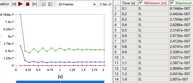
Maximum equivalent stress variation of fluid-structure coupling pile

According to the figure above, under the action of bidirectional fluid-structure interaction [16], the maximum equivalent stress at the bottom of a single row pile varies periodically from 2.4 EPa to 2.9 EPA within a certain time range. The tensile yield limit of the steel material is 2.5 EPA, which is within this rangeand the maximum equivalent stress variation range conforms to Von Mises yield criterion: when the equivalent stress of a point in the stressed object reaches a certain value, the point begins to enter the plastic state. Compared with the study of single pile by Zhang Shaobenji et al., it is shown that in a reasonable wave field, both single pile and single row pile are stable under the wave action, which has certain reference value for the stability design of pile under actual complex working conditions. Further research is needed for more complex multi-row piles under the same conditions.

3. Conclusion Analysis

1) Through the verification of the numerical wave tank model, the simulation value of the wave surface duration curve agrees well. Therefore, it is feasible to apply the wave numerical model to conduct a two-way flow-solid coupling analysis between wave and pile column.

2) This paper comprehensively considers the influence of the structure on the flow field, and obtains the relatively accurate calculation results.

3) The fluctuation range of the two-way flow-solid coupling velocity changes periodically, indicating that the deformation factors of the flow field cannot be ignored. The deformation of the pile column will cause the change of the flow field, and the bidirectional flow-solid coupling is more in line with the actual situation.

4) Through the bidirectional flow-solid coupling simulation of the pile column and the wave, the maximum stress of the pile column occurs at the bottom of the pile column.

5) The variation range of the maximum equal effect force of the single pile and the single row pile is within the tensile yield limit (Take the default tensile yield limit of the steel material_s = 2. 5 × 10⁸ Pa).

6) ANSYS-Workbench can well simulate the interaction between the flow field and the structure, and this study provides some basis for the stability design of marine platforms. The main direction of future research work is the other complex structures of marine platforms.

Conflicts of Interest

The authors declare no conflicts of interest regarding the publication of this paper.

References

[1]	Liu, X., Tan, G.H. and Wang, D.G. (2010) Numerical Generation of Second-Order Stokes Wave Based on Boundary Wave. Journal of Liaoning University of Engineering and Technology, 29, 107-111.
[2]	Liu, Y.F., Huang, X.F. and Lin, J.H. (1990) Structural and Mechanical Calculation of Dynamic Safety Calibration. Computational Structural Mechanics and Its Applications, 7, 73-83.
[3]	Hirt, C.W. and Nichols, B.D. (1981) Volume of Fluid Method of the Dynamics of Free Boundaries. Journal of Computational Physics, 39, 201-225. https://doi.org/10.1016/0021-9991(81)90145-5
[4]	Zhang, T. (2009) Three-Dimensional Numerical Simulation of Zhang Ting Wave and Its Application of Tianjin University. Ph.D. Thesis, Tianjin University, Tianjin. https://kns.cnki.net/KCMS/detail/detail.aspx?dbname=CMFD2011&filename=2010090758.nh
[5]	Liu, Z.Y., Zheng, Y., Zhang, W.J. and Si, J.J. (2009) ANSYS-CFX Methods Design. Water Resources and Hydropower Engineering, 28, 29-31.
[6]	Liu, Z.X., Song, B.J., Gu, C.G., et al. (1996) Numerical Study of the Higher-Order Anisotropic K-Model and Its Constant Coefficients. Journal of Engineering Thermophysics, 17, 31-34.
[7]	Liu, Y., Yong, Q., Zhang, H.Y. and Li, G. (2004) Analysis of the Wave Generation Process and Wave Morphology. Journal of Sichuan University, 36, 28-31.
[8]	Yang, J.P. (2006) Numerical Simulation of Wave Sink. Master’s Thesis, Harbin Engineering University, Harbin.
[9]	Zhang, Q.H., Zhang, J.F., Zhang, B.J. and Zhao, Y.F. (2011) Numerical Simulation Study of Wave Load of Offshore Fan Composite Cylinder Infrastructure. Collection of the Fifth National Hydraulics and Water Conservancy Informatics Conference, Tianjin, 13 October 2011, 448-454.
[10]	Bao, W.B. (2006) Numerical Simulation of Nonlinear Wave. Master’s Thesis, Dalian University of Technology, Dalian.
[11]	Yin, D.J. (2006) Study on Practical Model System of Coastal Wave. Master’s Dissertation, Hohai University, Nanjing.
[12]	Francesco, F. (2007) Explaining Extreme Waves by a Theory of Stochastic Wave Groups. Computers and Structures, 85, 291-303. https://doi.org/10.1016/j.compstruc.2006.10.007
[13]	Touboul, J. (2006) Freak Waves under the Action of Wind: Experiments and Simulations. European Journal of Mechanics B/Fluids, 25, 662-676. https://doi.org/10.1016/j.euromechflu.2006.02.006
[14]	Zhang, S.J., Zhu, X.L., Zhang, H. and Liu, Z.Y. (2014) Numerical Simulation of Bidirectional Flow-Solid Coupling between Single Pile Column and Wave. Water Resources and Hydropower Technology, 45, 63-66.
[15]	Guo, C.H. (2018) Bidirectional Fluid Solid Coupling Mechanism and Pulsation Absorption of Bionic Hydraulic Pipeline. Chinese Hydraulicsand Pneumatics, No. 9, 55-62.
[16]	Xie, L.H., Zhao, X.Y. and Zhang, J.M. (2012) ANSYS CFX Fluid Analysis and Simulation. Beijing Electronic Industry Press.