Simple Mitigation Strategy for a Systematic Gate Error in IBMQ

Daniel Bultrini, Max Hunter Gordon, Esperanza López, Germán Sierra

Instituto de Fsica Teórica, Universidad Autónoma de Madrid, Madrid, Spain.

DOI: 10.4236/jamp.2021.96083                

Abstract

In this paper, we report the observation and characterisation of a systematic error in the implementation of U₃ gates in the IBM quantum computers. By measuring the effect of this gate for various rotation angles the error appears as an over-rotation, whose magnitude does not correlate with IBM’s cited errors calculated using Clifford randomized benchmarking. We propose a simple mitigation procedure to limit the effects of this error. We show that using a simple mitigation strategy one can obtain improved results in the observed value for the CHSH inequality, measured in a cloud-based quantum computer. This work highlights the utility of simple mitigation strategies for short-depth quantum circuits.

Keywords

Quantum Computing, Error Mitigation, CHSH Inequalities

1. Introduction

The field of quantum computing has the potential to transform a wide variety of scientific fields including material science and quantum chemistry. Hardware noise in the computation presents a big problem for quantum computing as noise in general destroys coherence and entanglement in the quantum state, which is essential for a successful quantum algorithm. In order to address this problem, quantum error correction uses extra qubits to detect and correct errors introduced by the effects of noise. Error correction is essential in the development of fully functional quantum computers. However, existing hardware does not meet the requirements to implement fault-tolerant quantum error correction, outside of small preliminary studies [1] [2] [3] [4]. The accuracy of observables produced by current hardware is therefore limited, but many candidate applications require greater precision to outperform classical methods. For this reason, it is widely regarded that error mitigation will be essential in demonstrating near-term quantum advantage [5].

Error mitigation aims to reduce the effect of noise rather than remove it completely. There are many distinct approaches towards this goal, with two common methods being: optimizing quantum circuits through compilation and machine learning [6] [7] [8] and classical post-processing. One of the most promising post-processing techniques is zero noise extrapolation [9] which combines observables evaluated at several controlled noise levels [10] [11], enabling extrapolation to the zero-noise limit. Recently several new mitigation methods have been developed that make use of learning from data sets constructed using quantum circuit data [12] [13] demonstrating the rapid progress in this field.

Errors occur due to a multitude of factors in both the qubits themselves and the control hardware. Qubits are not completely isolated from their environment, leading to thermal relaxation and the decoherence of their state. Gate errors result from miscalibration or imperfections in the control hardware and their interactions with the qubits. Furthermore, the readout procedure can misidentify or alter the final qubit state such that the measured value does not accurately reflect the collapsed state [14]. Despite the widespread success of error mitigation strategies most methods do not directly focus on the effect of imperfect control hardware, which motivates the approach we take in this work.

Here we present a remarkably simple technique to mitigate the effect of over-rotations in short-depth quantum circuits. The method is based on first running diagnostic circuits which quantify the error. Then, using the quantified error the experimenter can run a modified circuit of interest to mitigate the effect of the over-rotation. We show that simple approaches, such as that presented, here can still offer an experimental advantage when implemented in real quantum hardware.

First, we introduce the mathematical description of several basic single qubit. Then we show how over-rotations can be characterised and their effects mitigated. This is followed by a simple experimental demonstration of our method where we measure the CHSH inequalities in real quantum hardware using the IBM cloud quantum computing service. Finally, we present a discussion of our method and the results obtained as well as future directions.

A single qubit pure state can be represented as:

$|\psi \rangle =\cos \left(\frac{\theta }{2}\right)|0\rangle +{\text{e}}^{i\varphi }\sin \left(\frac{\theta }{2}\right)|1\rangle .$ (1)

which can be visualized as a point on the Bloch sphere at polar angle $\theta$ and azimuthal angle $\varphi$.

During computation, a given number of one and two qubit gates are performed on a set of qubits. In the zero-noise limit this has the effect of changing the state by some unitary operation U. Any unitary is decomposed into the physical gate set of the device, $\mathcal{S}$. When implemented in the IBMQ quantum computer this set is given by $\mathcal{S}=\left\{U_1\left(\omega \right)\mathrm{,}{R}_x\left(\pm \pi /2\right)\mathrm{,}CX\right\}$, where $\omega$ is any angle. The gate $U_1\left(\omega \right)$ is equivalent to $R_z\left(\omega \right)$ up to a global phase factor and is implemented virtually within IBMQ. This is achieved by using frame changes with near-perfect execution [15] which does not involve the action of any physical quantum gates. A general single qubit unitary

$U_3\left(\theta \mathrm{,}\varphi \mathrm{,}\lambda \right)=\left(\begin{array}{cc}\cos \left(\theta /2\right)& -{\text{e}}^{i\lambda }\sin \left(\theta /2\right)\\ {\text{e}}^{i\varphi }\sin \left(\theta /2\right)& {\text{e}}^{i\left(\lambda +\varphi \right)}\cos \left(\theta /2\right)\end{array}\right)\mathrm{,}$ (2)

can be decomposed as follows:

$U_3\left(\theta \mathrm{,}\varphi \mathrm{,}\lambda \right)=R_z\left(\varphi \right)R_x\text{}\left(-\frac{\pi }{2}\right)R_z\left(\theta \right)R_x\text{}\left(\frac{\pi }{2}\right)R_z\left(\lambda \right)\mathrm{,}$ (3)

where the $R_z$ gates are implemented virtually (VZ), and the $R_x\left(\pm \pi /2\right)$ by a pulse [16].

Once execution of the required gates is complete, the quantum computer measures the qubits, collapsing the state, and outputs the results. The computation is repeated and a vector of counts ${\stackrel{\to }{v}}_{exp}$, length 2ⁿ (where n is the number of qubits), is obtained. Relaxation, imperfect coupling of the readout resonator and signal amplification lead to errors in the measurement process [14]. Although major improvements in this area are likely to come from improved hardware, it is possible to mitigate the measurement error through various techniques [17]. A simple strategy currently implemented within IBM’s Qiskit software [18] uses data from calibration circuits to mitigate the error using classical post-processing. This is achieved using the direct construction of a calibration matrix which for one qubit can be written as:

$M_{cal}=\left(\begin{array}{cc}{p}_0& 1-p_1\\ 1-p_0& p_1\end{array}\right)\mathrm{,}$ (4)

where $p_0$ and $p_1$ are the probabilities that a prepared $|0\rangle$ is measured as $|0\rangle$ and a prepared state $|1\rangle$ is measured as $|1\rangle$ respectively. This technique can be extended to multi-qubit states using a tensor product or correlated Markov noise approaches [19]. The calibration matrix can also be calculated using maximum likelihood techniques and quantum detector tomography [20].

The calibration matrix can then be used to mitigate errors associated with the readout either directly by: 1) inversion or through 2) bounded minimization.

1) Inversion is done by inverting the calibration matrix as such: $M_{cal}^{-1}{\stackrel{\to }{v}}_{exp}={\stackrel{\to }{v}}_{th}$, where ${\stackrel{\to }{v}}_{exp}\mathrm{,}{\stackrel{\to }{v}}_{th}$ are the experimental and ideal vectors of the counts.

2) Bounded minimization uses bounded least squares optimization: ${\min }_{{\stackrel{\to }{v}}_{th}}\left|M_{cal}{\stackrel{\to }{v}}_{th}-{\stackrel{\to }{v}}_{exp}\right|$, where bounds ensure the probabilities calculated from ${\stackrel{\to }{v}}_{th}$ are positive and correctly normalised.

These techniques share the assumption that the error rate in state preparation is much lower than the readout error. This is not without merit as single gate errors cited in IBM, Google and Rigetti are all below 0.5% while their readout errors are around 1% - 5% [14] [16] [21]. Yet, any error in state preparation, especially systematic ones, can lead to an inaccurate calibration matrix.

In this paper we highlight a systematic error in the execution of the U₃ gate in IBM’s cloud-based computers, which appears as a shift in the angle $\theta$ when implementing the gate $U_3\left(\theta \mathrm{,}\varphi \mathrm{,}\lambda \right)$. We propose to mitigate the previous error using an angular shift in $\theta$ in the U₃ gate. We illustrate the functionality of this mitigation method by measuring the CHSH inequality on data from a real device.

2. Error Characterisation

1) Sweeping a Meridian

To explore the reliability of the U₃ gate we applied it to the 0 state with $\lambda =\pi /2$, $\varphi =-\pi /2$ and various angles $\theta$ in the interval $\left[\mathrm{0,}\pi \right]$ (see Equation (2)).

This represents a rotation about the X axis ( $R_x\left(\theta \right)$ ) on the Bloch sphere that sweeps a whole meridian. The gate is followed by a measurement in the Z basis

IBM’s calibration method consists in measuring the states 0 and $|1\rangle =R_x\left(\pi \right)|0\rangle$, extracting the values of $p_0$ and $p_1$ to build the matrix $M_{cal}$ given in (4). The experimental 0 count for any given $\theta$ ( $P_0\left(\theta \right)$ ), ignoring all errors apart from readout, can be described by

$P_0\left(\theta \right)=p_0{\cos }^2\frac{\theta }{2}+\left(1-p_1\right){\sin }^2\frac{\theta }{2}\mathrm{.}$ (5)

We shall refer to this formula as the IBM-fit. Observe that (5) reproduces by construction the experimental data $p_0$ and $1-p_1$ for $\theta =0$ and $\pi$ respectively. To test the reliability of this formula we divide $\left[\mathrm{0,}\pi \right]$ in 30 intervals and measure $P_0\left({\theta }_i\right)$ for ${\theta }_i=\pi i/30$ with $i=0,1,\cdots ,30$. The results obtained for the qubit 9 of the Cambridge QC, with 8192 shots per angle, are plotted in Figure 1(a) together with the curve (5). One can easily see a significant deviation between the experimental data and the IBM prediction. However, this deviation follows a trend that we characterize with the following ansatz

$P_0\left(\theta \right)={p^{\prime }}_0{\cos }^2\frac{\theta +\alpha }{2}+\left(1-{p^{\prime }}_1\right){\sin }^2\frac{\theta +\alpha }{2}\mathrm{.}$ (6)

Figure 1. Sweep of $R_x\left(\theta \right)$ on Cambridge qubit 9. The raw data (blue dots) are fitted with the IBM method (red, dotted) and Shift-fit with $\alpha =-0.18$ (green, solid).

Here, the angle $\theta$ is shifted by a parameter $\alpha$ that takes small values, as we shall see below. The probabilities $p_0$ and $p_1$, appearing in (5), have been replaced by ${p^{\prime }}_0$ and ${p^{\prime }}_1$ to allow for a more accurate description of the experimental results in the range $\theta \in \left[\mathrm{0,}\pi \right]$. The numerical values of $\alpha \mathrm{,}{p^{\prime }}_0$ and ${p^{\prime }}_1$ are determined using a least-square fit of the set ${\left\{P_0\left({\theta }_i\right)\right\}}_{i=0}^{30}$ using Equation (6). We shall denote this approach as the Shift-fit method. Figure 2 shows that (6) provides a much better fit to the data than (5).

To quantify the performance of the fits we use the coefficient of determination R² that is defined as

$R_{\text{fit}}^2=1-\frac{{\displaystyle {\sum }_{n=0}^{30}{\left(P_0^{\text{exp}}\left({\theta }_n\right)-P_0^{\text{fit}}\left({\theta }_n\right)\right)}^2}}{{\displaystyle {\sum }_{n=0}^{30}{\left(P_0^{\text{exp}}\left({\theta }_n\right)-{\bar{P}}_0^{\text{exp}}\right)}^2}}$ (7)

where $P_0^{\exp }\left({\theta }_n\right)$ is the experimental probability of the $|0\rangle$ counts at angle ${\theta }_n$, and ${\bar{P}}_0^{\exp }$ its average. The R² estimator is customarily expressed in percentages, thus a perfect fit, implies a $R_{\text{fit}}^2\times 100=100\%$ of predictibilty. The data given in Figure 2 yield an R² equal to 97.6% for the IBM-fit and 99.9% for the Shift-fit.

2) Several Sweeps: Jobs

The results presented in Figure 1 correspond to a single sweep of equally spaced angles ${\theta }_n$ along a meridian.

To assess the reliability of the Shift-fit method we consider a set of $n_s$ consecutive sweeps that we denote a job. The number of sweeps $n_s$ can depend on the job (see Figure 2). A given job is run within a time lapse where the quantum computer is assumed to remain approximately under the same experimental conditions.

The result of each job is a set of parameters ${\left\{{\alpha }_s,{p^{\prime }}_{0,s},{p^{\prime }}_{1,s}\right\}}_{s=1}^{n_s}$, which according to the previous assumption, should be similar. Figure 3 shows the distribution of the values of $\alpha$ obtained for 15 jobs, amounting to a total of 100 sweeps. We notice that: 1) within each job the parameter $\alpha$ takes similar values, 2) the average value of $\alpha$ presents large deviations between jobs, as shown in the histogram.

Figure 2. A cartoon describing the way circuits, sweeps and jobs are implemented.

Figure 3. Distribution of fitted $\alpha$ values for 100 $R_x\left(\theta \right)$ sweeps for Cambridge qubit 9. The scatter plot shows the values of $\alpha$ per job over runtime, with the 15 different jobs with $n_s\in \left\{\mathrm{2,5,6,7}\right\}$ (100 sweeps) denoted by horizontal lines. The bottom displays a histogram of the data.

Item 1) is in rough agreement with the stability assumption made above, while item 2) can be attributed to different calibrations during the time delay between different jobs.

The distribution has a mean $\alpha$ of −0.14 (7), where the number in brackets is the standard deviation on the last digit shown. This mean does not properly reflect how $\alpha$ behaves within a single job, as for example the single run in Figure 1(a) whose $\alpha =-0.18$.

We also find that overall the average R² for the Shift-fit and IBM fit are 99.9% and 97.0% respectively leading to the conclusion that including an $\alpha$ shift results in a more accurate description of the raw data in general. Finally it is worth noting that we have not found correlation between the shift observed and IBM quoted errors.

In Table 1 we collect the results of the observed shift for a selection of qubits in the devices Paris, Johannesburg, Rochester, Cambridge and London. The chosen qubits are the ones that exhibit the highest average values of $\alpha$. The largest twenty average values are provided in the supplementary material.

We have also explored other meridians with our the Shift-fit method and found a negligible dependence on the meridian. Through testing the same qubits in the same job in all the computers with ten equally spaced $\varphi$ from 0 to $2\pi$ we saw a no shifts greater than the standard deviation from the mean and there was no trend of increase with a change in $\varphi$.

3) Mitigation

As explained above, the parameter $\alpha$ represents a systematic error that affects the rotation angle $\theta$ of the $U_3\left(\theta \mathrm{,}\varphi \mathrm{,}\lambda \right)$ gate. A naive way to mitigate it is to replace $\theta$ by $\theta -\alpha$, hoping that this displacement will compensate the error. The corresponding mitigated circuit is

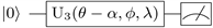
Table 1. Table showing average parameters from Equation (6) fitted to data from 100 sweeps over 10 jobs from different IBM quantum computers. Only qubits with the largest shift $\alpha$ are displayed. The standard deviation on the last digit is shown in round brackets after the mean value.

To implement the $\alpha$ mitigation a python software suite was written to perform these calibrations and implement the shift on subsequent experiments [22].

Figure 4 shows a selection of results. The values of $\alpha$, obtained with this type of mitigated circuit are much closer to zero that those obtained without the shift. The calibration and mitigated rotation were performed with a job with 10 sweeps. The R² values for the Shift-fit were above 99% in all cases. These results assess the effect of the mitigation method.

4) Repeated Gates and Different Initial States

We now explore the dependence of the $\alpha$ shift with the number of gates applied in a consecutive sequence. To this end we decompose a rotation $R_x\left(\theta \right)$ into M rotations of angle $\theta /M$, as shown in the circuit of Figure 5. The results for $M=1,\cdots ,10$ are given in Figure 6. We find that $\left|{\alpha }_M\right|$ increases with M, but not linearly as one would naively expect, that is ${\alpha }_M\simeq M{\alpha }_1$. All the tested computers returned different trends, and they changed between jobs even for the same computer. Sometimes a negative $\alpha$ would go closer to zero or further from zero and a positive $\alpha$ would sometimes grow or decrease. This fact suggests that the systematic error expressed by $\alpha$ has a complex origin that probably involves several components of the machine.

We have also studied sweeps starting, not from $|0\rangle$, but from the states obtained acting on $|0\rangle$ with $R_x\left(\pi /4\right)$, $R_x\left(\pi /2\right)$ and $R_x\left(3\pi /4\right)$. The results plotted in Figure 7, show a rough agreement of the values of $\alpha$. This suggests the result is not strongly state dependent.

3. Origin of the Error

In this section we propose an explanation of the shift-fit effect based on a potential error in the implementation of the gates $R_x\left(\pm \pi /2\right)$. In the ideal case these gates are realized as ${\text{e}}^{\mp it\Omega /2{\sigma }_X}$, where $\Omega$ is the pulse amplitude and $\Omega t=\pi /2$. An off resonance error (ORR) in the $R_x$ gate pulse can be modeled as follows [15]:

Figure 4. Box plot of the Shift ( $\alpha$ ) determined before (white) and after (blue) mitigation for a subset of qubits from several computers. The box and whiskers encompass 50% and 95% of the results respectively, dots represent outliers. Discrepancies between the data displayed here and that shown in Table 1 are due to it being run within different jobs. Furthermore some qubits are missing as they exhibited very small $\alpha$ values at runtime.

Figure 5. Repeated application of rotation gate $R_x\left(\theta /M\right)$ to complete at full $\theta$ rotation.

Figure 6. Distribution of ${\alpha }_M$ using the circuits shown in Figure 5. We perform 10 sweeps for each value of $M=1,\cdots ,10$, on the Cambridge qubit 9. The R² value does not appreciably decrease when increasing M, implying the fit stays consistent.

Figure 7. Distribution of $\alpha$ values starting the sweep from various initial states on Cambridge qubit 9. We employ 10 sweeps per state. The observed trend is not fully consistent between computers or qubits, hence the state dependence is not consistent.

$\begin{array}{c}{R}_x\left(\pm \pi /2\mathrm{,}\delta \right)=\exp \left[\frac{i\pi }{4}\left(\mp {\sigma }_X+\delta {\sigma }_Z\right)\right]\\ =\left(\begin{array}{cc}\cos \frac{\pi d}{4}-\frac{i\delta }{d}\sin \frac{\pi d}{4}& \mp \frac{i}{d}\sin \frac{\pi d}{4}\\ \mp \frac{i}{d}\sin \frac{\pi d}{4}& \cos \frac{\pi d}{4}+\frac{i\delta }{d}\sin \frac{\pi d}{4}\end{array}\right)\end{array}$ (8)

where $d=\sqrt{1+{\delta }^2}$. Replacing these gates into (3) we obtain a gate $U_3\left(\theta \mathrm{,}-\frac{\pi }{2}\mathrm{,}\frac{\pi }{2}\mathrm{,}\delta \right)$ that includes the ORR error. Finally, we apply the calibration matrix $M_{cal}$, to obtain the probability of measuring the $|0\rangle$ state for various angles $\theta$

$P_0^{\text{ORR}}\left(\theta ,\delta \right)=\frac{1+p_0-p_1}{2}+\frac{p_0+p_1-1}{2}\left[\left(1-2{\delta }^2\right)\cos \theta -2\delta \sin \theta \right]+O\left({\delta }^3\right),$ (9)

where we have assumed that $\delta$ is a small parameter. Starting from Equation (6) and expanding in powers of $\alpha$ gives

$P_0^{\text{shift}}\left(\theta \mathrm{,}\delta \right)=\frac{1+p_0-p_1}{2}+\frac{p_0+p_1-1}{2}\left[\left(1-\frac{{\alpha }^2}{2}\right)\cos \theta -\alpha \sin \theta \right]+O\left({\alpha }^3\right)\mathrm{.}$ (10)

These two expressions are equivalent up to $O\left({\delta }^3\right)$ assuming $\alpha =2\delta$ and the using the same calibration matrix. This means that the VZ gates can indeed be used to correct for this by replacing the $\theta$ parameter in Equation (3) with $\theta -\alpha$, which is equivalent to altering the $\theta$ in the U₃ gate.

It appears that the shift observed is well described by the appearance of ORR errors in the $R_x$ gates. However, upon multiple action of these gates, one would expect the errors to accumulate, resulting in a shift that grows proportionally with the number of applied gates. As previously demonstrated, this is not observed (see Figure 6).

We shall show that despite the previous complications, the $\alpha$ mitigation improves observed CHSH inequalities, suggesting the simple mitigation strategy we present could be useful in short-depth circuits.

4. Evaluating the CHSH Inequality

The CHSH inequality involves running 4 separate circuits which each consist of a Bell state preparation followed by measurements in four appropriately chosen bases (Figure 8). It is a quintessential experiment in quantum mechanics demonstrating that quantum correlations cannot be explained classically [23]. The correlation function can be expressed as follows:

Figure 8. CHSH circuit, $M_0$, $M_1$ represent the gates required for the basis changes to go into the $A_0{B}_1$, $A_0{B^{\prime }}_1$, ${A^{\prime }}_0{B}_1$ and ${A^{\prime }}_0{B^{\prime }}_1$ bases in order to measure $A=Z$, $A^{\prime }=X$, $B=1\sqrt{2}\left(X+Z\right)$ and $B^{\prime }=1\sqrt{2}\left(-X+Z\right)$.

Table 2. Shift values and correlation functions showing raw and $\alpha$ mitigated implementations of the CHSH inequality circuits for 819,200 shots per basis. Qubits with local connectivity were chosen to minimize the depth of the circuits necessary. The calibration of $\alpha$ was calculated with 10 repetitions. In all cases where there is a significant shift we see either a statistical improvement in the measured value for C.

$C=\langle AB\rangle +\langle A{B}^{\prime }\rangle +\langle A^{\prime }B\rangle -\langle A^{\prime }{B}^{\prime }\rangle$ (11)

where 4 system observables are shown as $A\mathrm{,}{A}^{\prime }$ and $B\mathrm{,}{B}^{\prime }$, these letters simply represent different measurement bases of the bipartite system comprising of A and B. $\langle AB\rangle$ is the correlated expectation for two of those observables. For a system with a hidden variable or classical correlations, $\left|C\right|$ is bounded at 2. For a system with maximal entanglement, this bound is $2\sqrt{2}$ [24].

In general the measured mitigated correlations are closer to the theoretical limit as in Table 2, with the least improved cases appearing when $\alpha$ is very small in one or both qubits. Therefore, using a simple mitigation strategy can improve measured quantities in a real device.

How this improvement scales with depth and number of qubits in the circuit is an important consideration. We have shown the shift effect does not appear to be consistent with increasing depth as seen in 6. However, when increasing the system size a set of calibration circuits could be run on each qubit to determine the $\alpha$ shift whose effect could then be mitigated as outlined above.

5. Discussion and Conclusions

In this paper, we have highlighted the existence of a systematic error, which appears as an angular shift ( $\alpha$ ) in the parameter $\theta$ of the U₃ gate, and demonstrated its effects can be mitigated by performing a simple calibration before running a set of jobs. This shift was shown to bare characteristics of an ORR error. Therefore, it is now possible to mitigate this component of the total error irrespective of the readout error and other errors. This leads to an increased performance on our benchmark circuits to calculate the CHSH inequality. We found that the systematic shifts are consistent over the time span of a few successive jobs, but not over larger stretches of time.

As the ORR error can be corrected through the use of VZ gates, the change in the $\theta$ parameter of the U₃ gate does just this [15]. Although using the “open pulse” capabilities of some IBMQ quantum computers and finely tuning the $R_x$ pulses would result in similar improvements, this is a more complicated procedure and may not completely remove the ORR effect.

We have also shown that although these errors can be corrected for single gates, the application of multiple gates to a single qubit does not follow the expected relation from the ORR treatment which implies a linear growth in the shift with multiple gates. This remains an open question on whether the gates are state-dependent or if other errors come into play once the qubit is not in the ground state and further investigation is left to future work. Despite this, applying this correction still yielded improved results in the CHSH inequalities.

Any simple mitigation strategy can only improve the fidelity of calculations by a small factor. Yet, a modest increase in fidelity for a small upfront computation may be worth the extra time. Although this method could not be applied to deep circuits we envision it could be useful for many qubit, short-depth quantum circuits, especially if combined with other mitigation techniques.

Acknowledgements

We would like to thank Diego Garca-Martn and Pol Forn for conversations. We also thank the IBM Quantum team for making multiple devices available via the IBM Quantum Experience. The access to the IBM Quantum Experience has been provided by the CSIC IBM Q Hub. We acknowledge support from La Caixa Foundation (DB, MHG), European Union’s Horizon 2020 research and innovation programme under the Marie Skodowska-Curie grant agreement No. 71367 (DB). MHG is supported by “la Caixa” Foundation (ID: 100010434), Grant No. LCF/BQ/DI19/11730056. This work has also been financed by the Spanish grants PGC2018-095862-B-C21, QUITEMAD + S2013/ICE-2801, SEV-2016-0597 of the “Centro de Excelencia Severo Ochoa” Programme and the CSIC Research Platform on Quantum Technologies PTI-001.

Supplementary Material

1) Coefficient of determination, R²

The coefficient of determination, R², is defined as

$R^2=1-\frac{S{S}_{\text{res}}}{S{S}_{\text{tot}}}$ (12)

where the total sum of squares $S{S}_{\text{tot}}$ and total sum of residuals $S{S}_{\text{res}}$ are

$S{S}_{\text{tot}}={\displaystyle \underset{i}{\sum }}{\left(y_i-\bar{y}\right)}^2$ (13)

$S{S}_{\text{res}}={\displaystyle \underset{i}{\sum }}{\left(y_i-f_i\right)}^2\mathrm{,}$ (14)

with $y_i$ being a particular data point, $f_i$ being the prediction of $y_i$ and $\bar{y}$ the average of the observed data. If $R^2=1$, the fit is an exact match to the experimental data while anything lower implies a progressively worse fit.

In total the statistics of the goodness of fit of our proposed shift with respect to IBM and the ideal curve (setting $p_0=p_1=1$ and $\alpha =0$ ) are tabulated below for an aggregate of all of the sweeps over all computers.

Furthermore the way that we ascertained that there was no correlation between the alpha values and the cited IBM error rate is that we ordered the size of the errors for a given computer’s qubits by magnitude and compared it to the magnitude of $\alpha$ associated with a given error rate’s job and there was no polynomial (up to order 4) which gave any appreciable R² value for any computer.

2) Largest observed shift values

The TableS1 below shows the fitted data for 20 qubits with the largest average $\alpha$ after 100 sweeps, with exception of Rochester at 10 sweeps due to the large number of qubits. This process was carried out on the Cambridge, London, Rochester, Paris and Johannesburg computers.

Table S1. Largest 20 shift values found in the computers that were investigated. The parameters correspond to those shown in Equation (6). This was repeated 10 times and errors show the standard deviation, with the error in the last digit shown in brackets.

Conflicts of Interest

The authors declare no conflicts of interest regarding the publication of this paper.

References

[1]	Campagne-Ibarcq, P., Eickbusch, A., Touzard, S., Zalys-Geller, E., Frattini, N.E., Sivak, V.V., et al. (2020) Quantum Error Correction of a Qubit Encoded in Grid States of an Oscillator. Nature, 584, 368-372. https://doi.org/10.1038/s41586-020-2603-3
[2]	Waldherr, G., Wang, Y., Zaiser, S., Jamali, M., Schulte-Herbrüggen, T., Abe, H., Ohshima, T., Isoya, J., Du, J.F., Neumann, P. and Wrachtrup, J. (2014) Quantum Error Correction in a Solid-State Hybrid Spin Register. Nature, 506, 204-207. https://doi.org/10.1038/nature12919
[3]	Kelly, J., Barends, R., Fowler, A. G., Megrant, A., Jeffrey, E., White, T.C., et al. (2015) State Preservation by Repetitive Error Detection in a Superconducting Quantum Circuit. Nature, 519, 66-69. https://doi.org/10.1038/nature14270
[4]	Cramer, J., Kalb, N., Rol, M.A., Hensen, B., Blok, M.S., Markham, M., Twitchen, D.J., Hanson, R. and Taminiau, T.H. (2016) Repeated Quantum Error Correction on a Continuously Encoded Qubit by Real-Time Feedback. Nature Communications, 7, Article No. 11526. https://doi.org/10.1038/ncomms11526
[5]	Preskill, J. (2018) Quantum Computing in the NISQ Era and Beyond. Quantum, 2, Article No. 79. https://doi.org/10.22331/q-2018-08-06-79
[6]	Cincio, L., Subaşı, Y., Sornborger, A.T. and Coles, P.J. (2018) Learning the Quantum Algorithm for State Overlap. New Journal of Physics, 20, Article ID: 113022. https://doi.org/10.1088/1367-2630/aae94a
[7]	Murali, P., Baker, J.M., Javadi-Abhari, A., Chong, F.T. and Martonosi, M. (2019) Noise-Adaptive Compiler Mappings for Noisy Intermediate-Scale Quantum Computers. Proceedings of the 24th International Conference on Architectural Support for Programming Languages and Operating Systems, Providence, April 2019, 1015-1029. https://doi.org/10.1145/3297858.3304075
[8]	Cincio, L., Rudinger, K., Sarovar, M. and Coles, P.J. (2020) Machine Learning of Noise-Resilient Quantum Circuits. PRX Quantum, 2, Article ID: 010324. https://doi.org/10.1103/PRXQuantum.2.010324
[9]	Temme, K., Bravyi, S. and Gambetta, J.M. (2017) Error Mitigation for Short-Depth Quantum Circuits. Physical Review Letters, 119, Article ID: 180509. https://doi.org/10.1103/PhysRevLett.119.180509
[10]	Dumitrescu, E.F., McCaskey, A.J., Hagen, G., Jansen, G.R., Morris, T.D., Papenbrock, T., Pooser, R.C., Dean, D.J. and Lougovski, P. (2018) Cloud Quantum Computing of an Atomic Nucleus. Physical Review Letters, 120, Article ID: 210501. https://doi.org/10.1103/PhysRevLett.120.210501
[11]	He, A., Nachman, B., de Jong, W.A. and Bauer, C.W. (2020) Zero-Noise Extrapolation for Quantum-Gate Error Mitigation with Identity Insertions. Physical Review A, 102, Article ID: 012426. https://doi.org/10.1103/PhysRevA.102.012426
[12]	Strikis, A., Qin, D., Chen, Y., Benjamin, S.C. and Li, Y. (2020) Learning-Based Quantum Error Mitigation. arXiv: 2005.07601 [quant-ph].
[13]	Czarnik, P., Arrasmith, A., Coles, P.J. and Cincio, L. (2020) Error Mitigation with Clifford Quantum-Circuit Data. arXiv: 2005.10189 [quant-ph].
[14]	Kjaergaard, M., Schwartz, M.E., Braumüller, J., Krantz, P., Wang, J.I.-J., Gustavsson, S. and Oliver, W.D. (2020) Superconducting Qubits: Current State of Play. Annual Review of Condensed Matter Physics, 11, 369-395. https://doi.org/10.1146/annurev-conmatphys-031119-050605
[15]	McKay, D.C., Wood, C.J., Sheldon, S., Chow, J.M. and Gambetta, J.M. (2017) Efficient Z Gates for Quantum Computing. Physical Review A, 96, Article ID: 022330. https://doi.org/10.1103/PhysRevA.96.022330
[16]	Abraham, H., Akhalwaya, I.Y., Aleksandrowicz, G., Alexander, T., Alexandrowics, G., Arbel, E., Asfaw, A., et al. (2019) Qiskit: An Open-source Framework for Quantum Computing (Version 0.7.2). Zenodo. http://doi.org/10.5281/zenodo.2562111
[17]	Maciejewski, F.B., Zimboras, Z. and Oszmaniec, M. (2020) Mitigation of Readout Noise in Near-Term Quantum Devices by Classical Post-Processing Based on Detector Tomography. Quantum, 4, 257. https://doi.org/10.22331/q-2020-04-24-257
[18]	Team, I.Q. (2019) Qiskit Tutorials: Measurement Error Mitigation.
[19]	Bravyi, S., Sheldon, S., Kandala, A., Mckay, D.C. and Gambetta, J.M. (2020) Mitigating Measurement Errors in Multiqubit Experiments. Physical Review A, 103, Article ID: 042605. https://doi.org/10.1103/PhysRevA.103.042605
[20]	Chen, Y., Farahzad, M., Yoo, S. and Wei, T.-C. (2019) Detector Tomography on IBM Quantum Computers and Mitigation of an Imperfect Measurement. Physical Review A, 100, Article ID: 052315. https://doi.org/10.1103/PhysRevA.100.052315
[21]	Rigetti Computing. https://rigetti.com/
[22]	(2020) Alice and Bob. https://gitlab.ift.uam-csic.es/danielbultrini/AB
[23]	Clauser, J.F., Horne, M.A., Shimony, A. and Holt, R.A. (1969) Proposed Experiment to Test Local Hidden-Variable Theories. Physical Review Letters, 23, Article No. 880. https://doi.org/10.1103/PhysRevLett.23.880
[24]	Cirel’son, B.S. (1980) Quantum Generalizations of Bell’s Inequality. Letters in Mathematical Physics, 4, 93-100. https://doi.org/10.1007/BF00417500