A Study of Banach Fixed Point Theorem and It’s Applications

Abstract

This paper aims at treating a study of Banach fixed point theorem for mapping results that introduced in the setting of normed space. The classical Banach fixed point theorem is a generalization of this work. A fixed point theory is a beautiful mixture of Mathematical analysis to explain some conditions in which maps give excellent solutions. Here later many mathematicians used this fixed point theory to establish their results, see for instance, Picard-Lindel of Theorem, The Picard theorem, Implicit function theorem etc. Also, we developed ideas that many of known fixed point theorems can easily be derived from the Banach theorem. It extends some recent works on the extension of Banach contraction principle to metric space with norm spaces.

Share and Cite:

Mannan, M. , Rahman, M. , Akter, H. , Nahar, N. and Mondal, S. (2021) A Study of Banach Fixed Point Theorem and It’s Applications. American Journal of Computational Mathematics, 11, 157-174. doi: 10.4236/ajcm.2021.112011.

1. Introduction

It is conventional to this work motivated by some recent work on Banach fixed point theorem for mappings defined on metric spaces with a partial order or a graph. One of the most important theorems is the Banach fixed point theorem and it is related to a complete normed space. The study on Banach Fixed Point Theorem and its Applications is a motivation of the development of Banach fixed point theorem. Polish Mathematician Stefan Banach had discussed Banach fixed point theorem as a part of his PhD thesis in 1922. Here, Banach contraction principle and Banach fixed point theorem is important for nonlinear analysis. It’s a modification of the ε-variational principle of Ekeland ( [1] [2] ) which is a crucial tool in nonlinear analysis like optimization, variational inequalities, differential equations, and control theory. After that, Banach fixed point theorem has been generalized and extended in several directions (i.e. [3] [4] [5] and the related references there in). Here at present, we discussed Banach fixed point theorem in normed spaces where Banach fixed point theorem was in matric space [6]. Finally we have shown some important applications of Banach fixed point theorem.

2. Preliminaries

We will discuss Banach fixed point theorem in metric spaces with complete normed spaces and related topics.

Metric Space [7]: Let X be a non-empty set. A mapping d : X × X is called a metric if x , y , z X the following properties are satisfied:

1) d ( x , y ) 0 .

2) d ( x , y ) = 0 if and only if x = y .

3) d ( x , y ) = d ( y , x ) [Symmetry].

4) d ( x , y ) d ( x , z ) + d ( z , y ) [Triangle inequality].

The set X together with metric d, then it is called a metric space. It is denoted by d ( X , d ) .

Example: A trivial but important example a metric is given by the function

d ( x , y ) = { 0 if x = y 1 if y y ; x , y X

Convergence and limit of a sequence: A sequence x n in a metrics space ( X , d ) is said to be convergent if there exist an x X such that

lim n d ( x n , x ) = 0 .

Here x is called the limit of x n and we write this as lim n x n = x .

Complete metric space: A metric ( X , d ) is said to be complete if every Cauchy sequence in it converges to an element of it.

Cauchy sequence: Let ( X , d ) be a metric space and ( x n ) be a sequence in it. Then the sequence ( x n ) is said be a Cauchy sequence if for every ϵ > 0 , there exists positive integer N such that d ( x p , x q ) < ϵ for all p , q > N

Complete Cauchy sequence:

Let ( X , d ) be a g.m.s. A sequence x n , n N in X is said to be a Cauchy sequence if for all ϵ > 0 there exists a natural number n ϵ N such that for all m , n N , n n ϵ one has d ( x n , x n + m ) < ϵ . ( X , d ) is called complete if every Cauchy sequence is convergent in X.

Fixed point: A fixed point of a mapping f : X X is a point x X such that f ( x ) = x .

Example:

1) The mapping x x 2 of into itself has the two fixed points 0 and 1.

2) A rotation of the plane has a single fixed point.

3) A translation has no fixed point.

Contraction mapping in metric space: Let ( X , d ) be a metric space. A mapping T : X X is called a contraction on X if there is a positive real number k < 1 such that for all x , y X .

d ( T x , T y ) k d ( x , y )

Normed Spaces [8]: A normed on X is a real function : X R defined on X such that for any x , y X and for all λ K .

1) x 0 .

2) x = 0 if and only if x = 0 .

3) λ x = | λ | x .

4) x + y x + y (Triangle inequality).

A norm on X defines a metric d on X which is given by d ( x , y ) = x y ; x , y X and is called the metric induced by the norm. The normed space is denoted by ( X , ) or simply by X.

Convergence: A sequence ( x n ) in a normed space X is said to be convergent if X contains an x such that lim n x n x = 0 . Then we write x n x . And call x is called the limit of x n .

Cauchy sequence: A sequence ( x n ) in a normed space X is called a Cauchy sequence if for every ε > 0 there exists a positive integer N such that

x n x < ε n , m > N

Banach Space [9]:

Definition-1: A complete normed space is called a Banach space. (Complete means complete in the metric defined by the norm.)

Definition-2: A normed space, in which every Cauchy sequence is convergent, is called a Banach space. That is, for every sequence ( x n ) in X with x m x n 0 as ( m , n ) , x X s.t. x n x 0 , as n .

Example-1: Every Banach space is a normed, but the converse, in general, is not true.

Example-2: R n and C n are Banach spaces with the norm definite by

x = ( l = 1 n | x 1 | 2 ) 1 / 2

Contraction mapping in norm space [10]: Let X be a norm space and T : X X . Then T is called a contraction mapping if there is a positive real number k < 1 such that for all x , y X . T ( x ) T ( y ) k x y .

3. Application with Result

Here, we present a Study of Banach Fixed Point Theorem and its Application’s for mapping results which is introduced in setting of normed spaces such as.

3.1. Banach Contraction Theorem (or Principle) [11]

Here we will give the proof of Banach contraction theorem (or principle) both for metric space and normed space separately.

Theorem-1: Let T be a contraction mapping on a complete metrice space X. Then T has a unique fixed point.

Proof: Let us consider an arbitrary point x 0 X and define the iterative sequence ( x n ) by

x 0 , x 1 = T x 0 , x 2 = T x 1 , x 3 = T x 2 , , x n = T x n 1 Then, x 2 = T T x 0 = T 2 x 0 x 3 = T T 2 x 0 = T 3 x 0 x n = T n x 0 } (1)

Then the sequence of the image of x 0 under repeated application of T. We now show that ( x n ) is a cauchy sequence.

If n > m , then

d ( x m + 1 , x m ) = d ( T x m , T x m 1 )

d ( x m + 1 , x m ) K d ( x m , x m 1 )

d ( x m + 1 , x m ) K d ( T x m 1 , T x m 2 )

d ( x m + 1 , x m ) K 2 d ( x m 1 , x m 2 )

Proceeding in this way up to m times we get,

d ( x m + 1 , x m ) K m d ( x 1 , x 0 )

Hence by the triangle inequality we obtain for n > m

d ( x m , x n ) d ( x m , x m + 1 ) + d ( x m + 1 , x m + 2 ) + + d ( x n 1 , x n ) K m d ( x 0 , x 1 ) + K m + 1 d ( x 0 , x 1 ) + + K n 1 d ( x 0 , x 1 ) = K m ( 1 + k + + k n m 1 ) d ( x 0 , x 1 ) = k m 1 k n m 1 K d ( x 0 , x 1 )

Since 0 < K < 1 , So that the number 1 k n m < 1

d ( x m , x n ) k m 1 K d ( x 0 , x 1 ) (2)

Again d ( x 0 , x 1 ) is fixed and 0 < K < 1 , so we can make the right hand side as small as we please by taking m sufficiently large. This shows that ( x n ) is a cauchy sequence.

Since X is complete, there exists a point x X Such that x n x . Now we show that this limit x is a fixed point of the mapping T. From triangle inequality and by definition we have

d ( x , T x ) d ( x , x n ) + d ( x n , T x )

d ( x , T x ) d ( x , x n ) + K d ( x n 1 , x )

We know that d ( x , y ) = 0 if and only if x = y . Since x n x , So d ( x , x n ) 0 and d ( x n 1 , x ) 0 . It follows that d ( x , T x ) = 0 and hence T x = x . This shows that x is a fixed point of T. We now show x is the only fixed point of T. Suppose that x 1 is also fixed point of T. Then T x 1 = x 1 .

d ( x , x 1 ) = d ( T x , T x 1 ) k d ( x , x 1 )

Since k < 1 , this implies that d ( x , x 1 ) = 0 . Hence x = x 1 . Thus, the proof is complete.

3.2. Hahna-Banach Theorem (Normed Space) [12] [13]

Let f be a bounded linear functional on a subspace Z of a normal space X. Then there exists a bounded linear functional F on X which is an extension of f to X and has the same norm.

F x f z (3)

where F x = sup x X | F ( x ) | , f z = sup x X x = 1 | f ( x ) |

Proof: If z = { 0 } , then f = 0 , and the extension F = 0 . Suppose Z { 0 } : For all x Z we have

| f ( x ) | = f z x

From the generalized Hahn-Banach theorem we have

| f ( x ) | p ( x ) .

Thus, p ( x ) can be taken as f z x , that is

p ( x ) = f z x (4)

We see that p is defined on all of X. We have

p ( x + y ) = f z x + y

p ( x + y ) = f z ( x y ) [By triangle inequality]

p ( x + y ) = f z x + f z y

p ( x + y ) = p ( x ) + p ( y )

and

p ( α x ) = f z α x = α f z x = | α | p ( x )

Hence by generalized Hahn-Banach theorem we can conclude that there a linear exists a linear functional F on X which is an extension of f and satisfies

| F ( x ) | p ( x ) = f z x x X

Taking the supremum over all x X of norm 1, we get

sup x X x = 1 | F ( x ) | f z

F x f z (5)

Since under an extension the norm can not decrease, so we have

F x f z (6)

From (5) and (6), then we get, F x = f z . Thus the theorem is proved.

Theorem-2: Let X be a normed space. Then the following mapping is all continuous.

1) ( x , y ) X × X x + y X

2) ( λ , x ) K × X λ x K

3) ( x , y ) X × X d ( x , y ) = y x R

Proof: 1) Let ( a , b ) X × X be an arbitrary point, so that a + b is its image. Now we will prove that the mapping is continuous at (a, b). I.e. for given ε > 0 , δ > 0 such that ( x + y ) ( a + b ) < ε Whenever x a < δ and

y b < δ . Let us take δ = 1 2 ε . Then we have

( x + y ) ( a + b ) = ( x a ) + ( y b )

( x + y ) ( a + b ) x a + y b

( x + y ) ( a + b ) < δ + δ

( x + y ) ( a + b ) < ε 2 + ε 2

( x + y ) ( a + b ) < ε

2) Let α K and a X be arbitrary. Now we will prove that the mapping is continuous at (α, a). I.e. for given ε > 0 , δ > 0 such that

λ x α a < ε

whenever λ α < δ and x a < δ we have the identity,

λ x α a = ( λ α ) ( x a ) + λ a + α x α a α a

λ x α a = ( λ α ) ( x a ) + ( λ α ) a + ( x a ) α

λ x α a = ( λ α ) ( x a ) + ( λ α ) a + ( x a ) α

Taking norm and using triangle inequality we get

λ x α a ( λ α ) ( x a ) + ( λ α ) a + ( x a ) α

λ x α a | λ α | x a + | λ α | a + | α | x a

Now choosing δ > 0 sufficiently small, we get

λ x α a δ δ + δ a + | α | δ < ε

λ x α a < ε

3) In this case, the function is the metric of a metric space. I follows from the property of metric spaces that the metric is continuous.

3.3. Banach Contraction Principle [14]

Every contraction mapping T defined on a Banach space X into itself has a unique fixed point x X .

Proof:

1) Existence of a fixed point:

Let us consider an arbitrary point x 0 X and define the interative sequence ( x n ) by x 0 , x 1 = T x 0 , x 2 = T x 1 , x 3 = T x 2 , , x n = T x n 1 . Then

x 2 = T T x 0 = T 2 x 0 x 3 = T T 2 x 0 = T 3 x 0 x n = T n x 0

It m > n , say m = n + p , p = 1 , 2 , . Then

x n + p x n = T n + p x 0 T n x 0 = T ( T n + p 1 x 0 T n 1 x 0 ) K T n + p 1 x 0 T n 1 x 0 ,

as T is a Contraction mapping Continuing this process this process n 1 times, we have

x n + p x n K n T p x 0 x 0 (7)

For n = 0 , 1 , 2 , 3 , and all p. Now,

T p x 0 x 0 = T p x 0 T p 1 x 0 + T p 1 x 0 T p 2 x 0 + T p 2 x 0 + T x 0 x 0

T p x 0 x 0 T p x 0 T p 1 x 0 + T p 1 x 0 T p 2 x 0 + + T x 0 x 0

T p x 0 x 0 T p 1 x 1 T p 1 x 0 + T p 2 x 1 T p 2 x 0 + + x 1 x 0

T p x 0 x 0 K p 1 x 1 x 0 + K p 2 x 1 x 0 + + x 1 x 0

T p x 0 x 0 ( K p 1 + K p 2 + + 1 ) x 1 x 0

T p x 0 x 0 1 K p 1 k x 1 x 0 (8)

by the sum of G.P. series whose ratio < 1. Since 0 < k < 1 , so the number 1 K p < 1 . Using this result in (8) we get

T p x 0 x 0 1 1 k x 1 x 0

with the help of this result (7) becomes

x n + p x n k n 1 k x 1 x 0

when n then m = n + p then

x n + p x n

This shows that ( x n ) is a cauchy sequence in X. Hence, ( x n ) must be convergent, say lim n x n = x

2) Limit x is a fixed points of T:

Since T is continuous, we have

T x = T ( lim n x n ) = lim n T x n = lim n x n + 1 = x

[Since the limit of ( x n + 1 ) is the same as that of ( x n ) ]

Thus, x is a fixed point of T.

3) Uniqueness of the fixed point:

Let y be another fixed point of T. Then, T y = y , We also have T x T y K x y , as T is contraction mapping. But T x T y x y . T x = x and T y = y x y K x y 1 K . Since 0 < K < 1 , So the above relation is possible only when

x y = 0

x y = 0

x = y

This proves that fixed point of T is unique.

Application-1: Let X = R be the Banach space of real numbers with x = | x | and [ a , b ] R , f : [ a , b ] [ a , b ] [ a , b ] , a differentiable function such that | f ( x ) | k < 1 . Find the solution of the equation f ( x ) = x .

Solution: Let x , y [ a , b ] and y < z < x . Then by Lagrange’s mean value theorem we have

f ( x ) f ( y ) x y = f ( z )

f ( x ) f ( y ) = ( x y ) f ( z )

| f ( x ) f ( y ) | = | ( x y ) f ( z ) |

| f ( x ) f ( y ) | = | x y | | f ( z ) |

| f ( x ) f ( y ) | k | x y |

Thus, f is a contraction mapping on [ a , b ] into itself. Since [ a , b ] is a closed subset of X = R . Therefore, by Banach contraction theorem exists a unique fixed point x * [ a , b ] such that f ( x * ) = x * . Hence, x * is the solution of the equation f ( x ) = x

Application-2:

Find the solution of the system of n linear algebraic equation with n unknowns:

a 11 x 1 + a 12 x 2 + + a 1 n x n = b 1 a 21 x 1 + a 22 x 2 + + a 2 n x n = b 2 a n 1 x 1 + a n 2 x 2 + + a n n x n = b n }

Solution:

The given system is

a 11 x 1 + a 12 x 2 + + a 1 n x n = b 1 a 21 x 1 + a 22 x 2 + + a 2 n x n = b 2 a n 1 x 1 + a n 2 x 2 + + a n n x n = b n } (9)

This system can be written as

x 1 = ( 1 a 11 ) x 1 a 12 x 2 a 1 n x n + b 1 x 2 = a 21 x 1 + ( 1 a 22 ) x 2 a 23 x 3 a 2 n x n + b 2 x n = a n 1 x 1 a n 2 x 2 + ( 1 a n n ) x n + b n } (10)

Let a i j = a i j + δ i j where δ i j = { 1 for i = j 0 for i j . Then the Equation (10) can be written in the following equivalent form.

x i = j = 1 n a i j x j + b , i = 1 , 2 , 3 , , n (11)

If x = ( x 1 , x 2 , , x n ) R n then Equation (11) can be written in the form T x = x , where T is defined by

T x = y (12)

where y = ( y 1 , y 2 , , y n ) and y i = j = 1 n a i j x j + b . Here T : R n R n and ( a i j ) is a n × n matrix.

Finding solutions of the system (9) or (11) is thus equivalent to find the fixed points of the operator (12). In order to find a unique fixed points of T, that is, a unique solution of (9), we apply the Banach contraction Principle, Equation (9) has a unique solution, if

j = 1 n | a i j | = j = 1 n | a i j + δ i j | K < 1 , i = 1 , 2 , , n

For

x = ( x 1 , x 2 , , x n ) R n

x = ( x 1 , x 2 , , x n ) R n

y = ( y 1 , y 2 , , y n ) R n

y = ( y 1 , y 2 , , y n ) R n

We have T x T x = y y

y i = j = 1 n α i j x j + b i , i = 1 , 2 , , n

Also if y = ( y 1 , y 2 , , y n ) R n then y = sup 1 i n | y i | . Therefore

T x T x = y y = sup 1 i n | y i y i | = sup 1 i n | j = 1 n a i j x j + b i j = 1 n a i j x j b i | = sup 1 i n | j = 1 n a i j ( x j x j ) |

T x T x sup 1 i n j = 1 n | a i j | | x j x j |

T x T x sup 1 i n j = 1 n | x j x j | sup 1 i n j = 1 n | a i j |

T x T x K sup 1 i n j = 1 n | x j x j | j = 1 n | a i j | k < 1

T x T x K x x x x = sup 1 i n | x j x j |

This shows that T a contraction mapping of the Banach space into itself. Hence, by Banach contraction principle, there exists a unique fixed point x * of T in R n , that is, x * is a solution of Equation (9).

Application-3:

Let the function K ( x , y ) be defined and measurable in the square

A = { ( x , y ) : a x b , a y b } .

Further, let a b a b | K ( x , y ) | 2 d x d y < , and g ( x ) L 2 ( a , b ) . Then the integral equation

f ( x ) = g ( x ) + λ a b K ( x , y ) f ( y ) d y (13)

has a unique solution f ( x ) L 2 ( a , b ) for every sufficiently small value of the parameter λ .

Proof: Let x = L 2 , and consider the mapping T

T : L 2 ( a , b ) L 2 ( a , b )

T f = h

where h ( x ) = g ( x ) = λ a b K ( x , y ) f ( y ) d y . This definition is valid for each f L 2 ( a , b ) , h L 2 ( a , b ) . Since g L 2 ( a , b ) and λ is a Scalar, it is sufficient to show that

ψ ( x ) = λ a b K ( x , y ) f ( y ) d y L 2 ( a , b )

By Cauchy –Schwartz inequality we have

| ψ ( x ) | = | a b K ( x , y ) f ( y ) d y |

| ψ ( x ) | a b | K ( x , y ) f ( y ) | d y

| ψ ( x ) | ( a b | K ( x , y ) | 2 d y ) 1 / 2 ( a b | f ( y ) | 2 d y ) 1 / 2

| ψ ( x ) | 2 ( a b | K ( x , y ) | 2 d y ) ( a b | f ( y ) | 2 d y )

a b | ψ ( x ) | 2 d x a b ( a b | K ( x , y ) | 2 d y ) d x a b ( a b | f ( y ) | 2 d y ) d x

By the hypothesis a b a b | K ( x , y ) | 2 d x d y < and a b ( a b | f ( y ) | 2 d y ) d x <

a b | ψ ( x ) | 2 d x <

Thus, ψ ( x ) = a b K ( x , y ) f ( x , y ) f ( y ) d y L 2 ( a , b ) . We know that L 2 ( a , b ) is a Banach space with norm

f = ( a b | f ( y ) | 2 d y ) 1 / 2

We now show that T is a contraction mapping. We have T f T f 1 = h h 1 .Where h 1 ( x ) = g 1 ( x ) + λ a b K ( x , y ) f 1 ( y ) d y . But,

h h 1 = g ( x ) + λ a b K ( x , y ) f ( y ) d y g 1 ( x ) λ a b K ( x , y ) f 1 ( y ) d y

h h 1 = [ g ( x ) g 1 ( x ) ] + λ a b [ K ( x , y ) { f ( y ) f 1 ( y ) } ] d y

h h 1 g ( x ) g 1 ( x ) + λ a b [ K ( x , y ) { f ( y ) f 1 ( y ) } ] d y

h h 1 λ a b [ K ( x , y ) { f ( y ) f 1 ( y ) } ] d y

h h 1 | λ | ( a b | [ a b K ( x , y ) { f ( y ) f 1 ( y ) } d y ] | 2 d x ) 1 / 2

h h 1 | λ | ( a b a b | K ( x , y ) | 2 d x d y ) 1 / 2 ( a b | f ( y ) f 1 ( y ) | 2 d y ) 1 / 2

[By using Cauchy –Schwartz-Bunyakowski inequality]

h h 1 | λ | ( a b a b | K ( x , y ) | 2 d x d y ) 1 / 2 f f 1

Hence, T f T f 1 | λ | ( a b a b | K ( x , y ) | 2 d x d y ) 1 / 2 f f 1 . If | λ | < 1 ( a b a b | K ( x , y ) | 2 d x d y ) 1 / 2 then

T f T f 1 K f f 1

where, K = | λ | ( a b a b | K ( x , y ) | 2 d x d y ) 1 / 2 < 1 .

Thus T is a contraction and so T has a unique fixed point. That is, there exists a unique f * L 2 ( a , b ) such that T f * = f * . This fixed point f * is a unique solution of the Equation (13).

Application-4: Show that the fredholm integral equation x ( s ) = y ( s ) + μ a b K ( s , t ) x ( t ) d t has a unique solution on [ a , b ]

Solution: We assume that K ( s , t ) is continuous in both variables a s b and a t b . Let y C [ a , b ] . Hence, | K ( s , t ) | λ for all ( s , t ) [ a , b ] × [ a , b ] . We first consider the integral equation on C [ a , b ] , the space of all Continuous defined on the interval [ a , b ] with the metric.

d ( x , y ) = max t [ a , b ] | x ( t ) y ( t ) |

Write the given integral equation in the form x = T x , where

T x ( s ) = y ( s ) + μ a b K ( s , t ) x ( t ) d t (14)

Since the kernel K and the function y are continuous, it follows that Equation (i) defines an operator

T : C [ a , b ] C [ a , b ]

It follows that

d ( T x , T y ) = max t [ a , b ] | T x ( t ) T y ( t ) | = max t [ a , b ] | y ( t ) + μ a b K ( s , t ) x ( t ) d t y ( t ) μ a b K ( s , t ) y ( t ) d t | = max t [ a , b ] | μ a b K ( s , t ) [ x ( t ) y ( t ) ] d t | = | μ | max t [ a , b ] | a b K ( s , t ) [ x ( t ) y ( t ) ] d t |

d ( T x , T y ) | μ | max t [ a , b ] a b | K ( s , t ) | | x ( t ) y ( t ) | d t

d ( T x , T y ) | μ | λ max t [ a , b ] | x ( u ) y ( u ) | a b d t

d ( T x , T y ) | μ | λ d ( x , y ) ( b a )

d ( T x , T y ) K d ( x , y ) , where K = | μ | λ ( b a )

If K < 1 | μ | λ ( b a ) < 1 | μ | < 1 λ ( b a ) , then T becomes contraction. Under this condition, we conclude that T has a unique solution x on [ a , b ] .

Application-5: Show that the Voltera integral equation on x ( s ) = y ( s ) + μ a b K ( s , t ) x ( t ) d t has a unique solution on | a , b | for every μ , where a t s and a s b

Solution: We notice that here a is fixed and s is variable limit of integration. Suppose that y is continuous on | a , b | and the kernel K ( s , t ) is continuous on the triangular region G in the s-t plane given by a t s , a s b

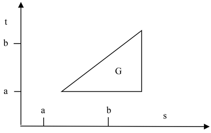
Writing the given equation as x = T x . Where T : C [ a , b ] C [ a , b ] . Defined by T x ( s ) = y ( s ) + μ a s K ( s , t ) x ( t ) d t . Since K ( s , t ) is continuous on and G is closed and bounded, it follows that | K ( s , t ) | c for all ( s , t ) G . We define the metric

d ( x , y ) = max t [ a , b ] | x ( t ) y ( t ) |

By using this metric we get

| T x ( s ) T y ( s ) | = | y ( s ) + μ a s K ( s , t ) x ( t ) d t y ( s ) μ a s K ( s , t ) y ( t ) d t | = | μ a s K ( s , t ) ( x ( t ) y ( t ) ) d t | = | μ | | a s K ( s , t ) ( x ( t ) y ( t ) ) d t | | μ | a s | K ( s , t ) | | x ( t ) y ( t ) | d t | μ | c max t [ a , b ] | x ( t ) y ( t ) | a b d t = | μ | c d ( x , y ) ( s a )

| T x ( s ) T y ( s ) | | μ | c ( s a ) d ( x , y )

By induction, now we will prove

| T m x ( s ) T m y ( s ) | | μ | m c m ( s a ) m m ! d ( x , y ) (15)

For n = 1 , the rersult holds, assume that this holds for n = m . Then

| T m + 1 x ( s ) T m + 1 y ( s ) | = | μ | | a s K ( s , t ) ( T m x ( t ) T m y ( t ) ) d t | | μ | a s | K ( s , t ) | | T m x ( t ) T m y ( t ) | d t | μ | c | μ | m c m a s ( t a ) m m ! d ( x , y ) d t | μ | m + 1 c m + 1 ( s a ) m + 1 ( m + 1 ) ! d ( x , y )

| T m + 1 x ( s ) T m + 1 y ( s ) | | μ | m + 1 c m + 1 ( s a ) m + 1 ( m + 1 ) ! d ( x , y )

This completes the inductive proof of (15). Using ( s a ) ( b a ) on the right hand side of (15) and then taking the maximum over t [ a , b ] on the left, we obtain from (15)

d ( T m x , T m y ) α m d ( x , y )

where α m = | μ | m c m ( b a ) m m ! .

For any fixed μ and sufficiently large m we have α m < 1 . Hence the corresponding T m is a contraction on C | a , b | .

Therefore, by Banach fixed theorem, T m has a fixed point x on [ a , b ] . We know that if T m has a fixed point, then T has the same fixed point. Thus T has a unique solution x on [ a , b ] .

Application-6: (Picards Theorem): Let f ( x , y ) be a continuous function of two variables in a rectangle, A = { ( x , y ) : a x b , c y d } and satisfy the Lipschitz condition in the second variable y.

Further, let ( x 0 , y 0 ) be any interior point of A. Then the differential Equation d y d x = f ( x , y ) has a unique solution, say y = g ( x ) which passes through ( x 0 , y 0 ) .

Proof: Given that the differential equation is

d y d x = f ( x , y ) (16)

Let y = g ( x ) satisfy (16) and the property that g ( x 0 ) = y 0 . Integrating (16) from x0 to x we get

[ y ] x 0 x = x 0 x f ( t , g ( t ) ) d t

g ( x ) g ( x 0 ) = x 0 x f ( t , g ( t ) ) d t [ y = g ( x ) ]

g ( x ) = y 0 + x 0 x f ( t , g ( t ) ) d t (17)

Thus a unique solution of (16) is equivalent to a unique solution of (17). Since f ( x , y ) satisfies the Lipshitz condition in y, there exists a constant q > 0 such that | f ( x , y 1 ) f ( x , y 2 ) | q | y 1 y 2 | where ( x , y 1 ) , ( x , y 2 ) A

The Rectangle A.

Since f ( x , y ) is continuous on a compact subset A of R2, it is bounded. So there exists a positive constant m such that | f ( x , y ) | m , ( x , y ) A . Let us choose a positive constant p such that p q < 1 and the rectangle.

B = { ( x , y ) | x 0 p x x 0 + p , y 0 p m y y 0 + p m }

is contained inA.

Let X be the set of all real –valued continuous functions y = g ( x ) defined on [ x 0 p , x 0 + p ] such that g ( x ) y 0 m p i.e. X is a closed subset of the Banach space C [ x 0 p , x 0 + p ] with the sup norm.

Let T : X X be defined as T g = h where h ( x ) = y 0 + x 0 x f ( t , g ( t ) ) d t . Here h ( x ) y 0 = x 0 x f ( t , g ( t ) ) d t

h ( x ) y 0 x 0 x | f ( t , g ( t ) ) | d t

h ( x ) y 0 m x 0 x d t

h ( x ) y 0 m ( x x 0 ) m p

h ( x ) X and so T is well defined. Let g , g 1 X . Then

T g T g 1 = h h 1 = y 0 + x 0 x f ( t , g ( t ) ) d t y 0 x 0 x f ( t , g 1 ( t ) ) d t = x 0 x ( f ( t , g ( t ) ) f ( t , g 1 ( t ) ) ) d t x 0 x f ( t , g ( t ) ) f ( t , g 1 ( t ) ) d t

q x 0 x g ( t ) g 1 ( t ) d t = q ( x x 0 ) g g 1 p q g g 1

T g T g 1 k g g 1 ,

where 0 < k = p q < 1 .

Hence, T is a contraction mapping of X onto itself. Therefore, by Banach contraction theorem, T has a unique fixed point g * X . This unique fixed point g * , is the unique solution of (17).

Problem-1: Let T : R R be defined by T ( x ) = x 2 . Determine the fixed point of T.

Solution:

Given that T ( x ) = x 2 . From the definition of fixed point we have,

T ( x ) = x

T ( x ) = x 2 = x

x 2 = x

x 2 x = 0

x ( x 1 ) = 0

x = 0 or x 1 = 0

x = 0 , 1

Thus the fixed points of T are 0 and 1.

Problem-2: Does a translation mapping T ( x ) = x + a where a is fixed have a fixed points.

Solution:

Given that T ( x ) = x + a . From the definition of fixed point we have,

T ( x ) = x

x + a = x + 0

a = 0 [By Left Cancellation Law]

Since T ( x ) = x + a is a translation mapping, so a 0 . Thus, the translation mapping T ( x ) = x + a has no fixed point.

Problem-3: Show that f ( x ) = x for x [ 2 , 1 ] [ 1 , 2 ] has no fixed po- int.

Solution:

Given that f ( x ) = x . From the definition of fixed point we have

f ( x ) = x

f ( x ) = x = x

It is clear that no point of [ 2 , 1 ] [ 1 , 2 ] will satisfy the Condition f ( x ) = x = x . Thus, f ( x ) = x has no fixed point x [ 2 , 1 ] [ 1 , 2 ] .

Problem-4: Let T be a mapping of R in to itself defined by T ( x ) = 1 2 x . Show that T has a unique fixed point.

Solution:

Given T ( x ) = 1 2 x

T ( y ) = 1 2 y

T ( x ) T ( y ) = 1 2 x 1 2 y = x y

Thus T is a contraction mapping. Hence, by Banach fixed point theorem, T has a unique fixed point.

Problem-5: Given an example to show that T satisfies T ( x ) T ( y ) = x y may not have any fixed point?

Solution:

Let T : R R be defined by

T ( x ) = { x 1 2 e x for x 0 1 2 + 1 2 x for x 0 (18)

T ( y ) = { y 1 2 e y for y 0 1 2 + 1 2 y for y 0 (19)

Now for x , y 0

T ( x ) T ( y ) = x 1 2 e x y + 1 2 e y = ( x y ) 1 2 ( e x e y ) x y

For x , y 0

T ( x ) T ( y ) = 1 2 + 1 2 x + 1 2 1 2 y = 1 2 ( x y ) x y

Thus T satisfies, T ( x ) T ( y ) x y . But from the definition of fixed point we have T ( x ) = x .

Now for x 0 .

T ( x ) = x = x 1 2 e x x = x 1 2 e x 0 = 1 2 e x e x = 0 = e 1

x = 1

This is not acceptable as x 0 .

For x 0

T ( x ) = x = 1 2 + 1 2 x x = 1 2 + 1 2 x 1 2 x = 1 2 x = 1

This is not acceptable as x 0 .

Thus, T defined in (18) is an example which satisfies the given condition (Banach contration theorem) but have no fixed point.

Again from the definition of fixed point we have

T ( y ) = y

Now for y 0

T ( y ) = y = y 1 2 e y y = y 1 2 e y 0 = 1 2 e y e y = 0 = e 1

y = 1

This is not acceptable as y 0 .

For y 0

T ( y ) = y = 1 2 + 1 2 y y = 1 2 + 1 2 y 1 2 y = 1 2 y = 1

This is not acceptable as y 0 .

Thus, defined in (19) is an example which satisfies the given condition (Banach contration theorem) but have no fixed point.

4. Conclusion

The Banach theorem seems somewhat limited. It seems intuitively clear that any continuous function mapping the unit interval into itself has a fixed point. We hope that this work will be useful for functional analysis related to normed spaces and fixed point theory. Our results are generalizations of the corresponding known fixed point results in the setting of Banach spaces on its norm spaces. Then all expected results in this paper will help us to understand better solution of complicated theorem. In future, we will discuss of Banach spaces on its norm spaces related properties to physical problem.

Acknowledgements

I would like to thank my respectable teacher Prof. Dr. Moqbul Hossain for encouragement and valuable suggestions.

Authors’ Contributions

Authors have made equal contributions for paper.

Conflicts of Interest

The authors declare that they have no competing interests.

References

[1] Ekeland, I. (1974) On the Variational Principle. Journal of Mathematical Analysis and Applications, 47, 324-353.
https://doi.org/10.1016/0022-247X(74)90025-0
[2] Ekeland, I. (1979) Nonconvex Minimization Problems. Bulletin of the American Mathematical Society, 1, 443-474.
https://doi.org/10.1090/S0273-0979-1979-14595-6
[3] Alfuraidan, M. and Ansari, Q. (2016) Fixed Point Theory and Graph Theory: Foundations and Integrative Approaches. Academic Press-Elsevier, London.
https://doi.org/10.1016/B978-0-12-804295-3.50013-9
[4] Guran, L. (2012) Ulam-Hyers Stability of Fixed Point Equations for Single Valued Operators on KST Spaces. Creative Mathematics Informatics, 21, 41-47.
https://doi.org/10.37193/CMI.2012.01.13
[5] Hasanzade Asl, J., Rezapour, S. and Shahzad, N. (2012) On Fixed Points of α-ψ-Contractive Multifunctions. Fixed Point Theory and Applications, 2012, Article No. 212.
https://doi.org/10.1186/1687-1812-2012-212
[6] Khojasteh, F., et al. (2016) Some Applications of Caristi’s Fixed Point Theorem in Metric Spaces. Fixed Point Theory and Applications, 2016, Article No. 16.
https://doi.org/10.1186/s13663-016-0501-z
[7] Khojasteh, F., Karapmar, E. and Radenovic, S. (2013) θ-Metric Space: A Generalization. Mathematical Problems in Engineering, 2013, Article ID 504609, 7 p.
https://doi.org/10.1155/2013/504609
[8] Rudin, W. (1991) Functional Analysis. Second Edition, International Editions, Mc-Graw-Hill, New York, ISBN 0-07-100944-2.
[9] Agarwal, R.P., Hussain, N. and Taoudi, M.-A. (2012) Fixed Point Theorems in Ordered Banach Spaces and Applications to Nonlinear Integral Equations. Abstract and Applied Analysis, 2012, Article ID: 245872, 15 p.
https://doi.org/10.1155/2012/245872
[10] Lu, N., He, F. and Huang, H. (2019) Answers to Questions on the Generalized Banach Contraction Conjecture in b-Metric Spaces. Journal of Fixed Point Theory and Applications, 21, 43.
https://doi.org/10.1007/s11784-019-0679-x
[11] Jain, S., Jain, S. and Jain, L.B. (2012) On Banach Contraction Principle in a Cone Metric Space. Journal of Nonlinear Sciences and Applications, 5, 252-258.
https://doi.org/10.22436/jnsa.005.04.01
[12] Jleli, M. and Samet, B. (2014) A New Generalization of the Banach Contraction Principle. Journal of Inequalities and Applications, 2014, Article No. 38.
https://doi.org/10.1186/1029-242X-2014-38
[13] Ferreira, M.A.M. and Andrade, M. (2011) Hahn-Banach Theorem for Normed Spaces. International Journal of Academic Research, 3, 13-16.
[14] Palais, R.S. (2007) A Simple Proof of the Banach Contraction Principle. Journal of Fixed Point Theory and Applications, 2, 221-223.
https://doi.org/10.1007/s11784-007-0041-6

Copyright © 2024 by authors and Scientific Research Publishing Inc.

Creative Commons License

This work and the related PDF file are licensed under a Creative Commons Attribution 4.0 International License.