Continuous-Time and Discrete-Time Singular Value Decomposition of an Impulse Response Function

Rogelio Luck, Yucheng Liu

Department of Mechanical Engineering, Mississippi State University, Mississippi State, MS, USA.

DOI: 10.4236/am.2021.124024                

Abstract

This paper proposes the continuous-time singular value decomposition (SVD) for the impulse response function, a special kind of Green’s functions, in order to find a set of singular functions and singular values so that the convolutions of such function with the set of singular functions on a specified domain are the solutions to the inhomogeneous differential equations for those singular functions. A numerical example was illustrated to verify the proposed method. Besides the continuous-time SVD, a discrete-time SVD is also presented for the impulse response function, which is modeled using a Toeplitz matrix in the discrete system. The proposed method has broad applications in signal processing, dynamic system analysis, acoustic analysis, thermal analysis, as well as macroeconomic modeling.

Keywords

Singular Value Decomposition, Impulse Response Function, Green’s Function, Toeplitz Matrix, Hankel Matrix

1. Introduction

Impulse response function (IRF) has been considerably used for signal processing, dynamic system analysis, acoustic analysis, thermal analysis, and macroeconomic modeling. The significance of such function is that for any input, the output can be calculated in terms of the input and the impulse response. To determine an output directly in the time domain requires the convolution of the input with the impulse response, which is very complicated. Therefore, it is usually to calculate the Laplace transform of a system’s output by the multiplication of the Laplace transform of the IRF with the input’s Laplace transform in the frequency domain at first; and then find the output in the time domain through an inverse Laplace transform.

This study proposes a direct method to calculate the system output through the singular value decomposition (SVD) algorithm. As a popular technique of factorizing a matrix, a variety of forms of SVD have been developed recently and applied for solving a wide range of scientific and engineering problems. For exam, Ramirez-Velarde et al. used SVD on the video correlation matrix to perform the principal component analysis [1]. Liu et al. developed an SVD-based minutia matching method for finger vein recognition, which performs better than other methods [2]. Wan et al. proposed a quasi SVD method to extract algebraic features from human face with enhanced face recognition rate and speed [3]. Zhang et al. applied a higher-order SVD method for denoising magnetic resonance data to improve the inspection quality and reliability of quantitative image analysis [4]. Shih et al. proposed an adaptive parametrized block-based SVD for preserving the edge structure and avoiding blurred image after the compressing process [5]. Ghazy et al. presented a block based watermarking scheme using the SVD algorithm to embed encrypted watermarks into digital images. Experimental results showed that the SVD-based method is superior to the traditional method for embedding encrypted watermarks and extracting them efficiently under attacks [6]. Cai et al. used SVD for model predictive control design of distribution systems and demonstrated the advantages of their method through two case studies [7]. Katsaounis et al. derived a new way to detect combinatorial equivalence of symmetric factorial designs based on the SVD of design matrices to provide a fast screen for non-equivalence [8]. Berenguer et al. used SVD of successive iterated solutions on subdomains interfaces to computing a low-rank approximation of the Aitken’s formula at a high computational efficiency. The results were then applied for solving heterogeneous 3D groundwater flow problems [9]. di Dio applied SVD for analyzing temperature dependent radial distribution functions and showed that the generality of the SVD approach allows investigating various temperature dependent structures in a unified way [10]. Abuturab proposed a new color image security system based on SVD in gyrator transform domains and proved robustness and other advantages of the developed method in enhancing the security [11]. Kavaklioglu applied SVD for modeling Turkey’s electricity consumption, in which the SVD was used to reduce the dimensionality of the problem and to provide robustness to the estimations [12]. However, in the previous studies, SVD was only applied for discrete systems (matrices) and this paper aims to present a continuous-time SVD approach for the first time to facilitate the calculation of convolution of a set of singular functions and the IRF ${\text{e}}^{-\left(t-\tau \right)}$.

2. Continuous-Time SVD of $e^{-\left(t-\tau \right)}$

Given an impulse response function (Green’s function) of the form:

$h\left(t,\tau \right)={\text{e}}^{-\left(t-\tau \right)}$

The analysis below shows how to find a set of “singular” functions $f\left(j,\tau \right)$ and singular values $D_j\left(j=0,1,2,\cdots \right)$ such that:

${\displaystyle {\int }_0^{t}h\left(t,\tau \right)f\left(j,\tau \right)\text{d}\tau }=D_{j}f\left(j,T-t\right),t\le T$ (1)

The left hand side of Equation (1) is Duhamel’s integral [13] for an input $f\left(j,t\right)$, where the $h\left(t,\tau \right)={\text{e}}^{-\left(t-\tau \right)}$.

Conjecture 1: $f\left(j,\tau \right)=\sin \left({\omega }_j\tau +{\varphi }_j\right)$

Proof

If conjecture 1 is correct, Equation (1) then becomes:

${\displaystyle {\int }_0^t{\text{e}}^{\tau }\sin \left({\omega }_j\tau +{\varphi }_j\right)\text{d}\tau }={\text{e}}^t{D}_j\sin \left[{\omega }_j\left(T-t\right)+{\varphi }_j\right],t\le T$ (2)

The complete solution process for Equation (2) includes three steps: 1) simplification of left hand side of Equation (2); 2) simplification of right hand side of Equation (2); 3) solve the simplified Equation (2).

Step 1: Simplifying ${\displaystyle {\int }_0^t{\text{e}}^{\tau }\sin \left({\omega }_j\tau +{\varphi }_j\right)\text{d}\tau }$

The integral on left hand side of Equation (2) can be solved as:

$\begin{array}{l}{\displaystyle {\int }_0^t{\text{e}}^{\tau }\sin \left({\omega }_j\tau +{\varphi }_j\right)\text{d}\tau }\\ =\frac{{\text{e}}^t\sin \left({\varphi }_j+{\omega }_{j}t\right)-{\omega }_j{\text{e}}^t\cos \left({\varphi }_j+{\omega }_{j}t\right)}{1+{\omega }_j^2}-\frac{\sin \left({\varphi }_j\right)-{\omega }_j\cos \left({\varphi }_j\right)}{1+{\omega }_j^2}\end{array}$ (3)

The first term on the right hand side of Equation (3) can be simplified as:

$\frac{{\text{e}}^t\sin \left({\varphi }_j+{\omega }_{j}t\right)-{\omega }_j{\text{e}}^t\cos \left({\varphi }_j+{\omega }_{j}t\right)}{1+{\omega }_j^2}={\text{e}}^t\frac{\sin \left({\varphi }_j+t{\omega }_j-\text{atan}\left({\omega }_j\right)\right)}{\sqrt{1+{\omega }_j^2}}$ (4)

In order to find ${\varphi }_j$ to satisfy Equation (3), the second term on the right hand side of that equation can be set to zero:

$\sin \left({\varphi }_j\right)-{\omega }_j\cos \left({\varphi }_j\right)=0$ (5)

Solutions of the above equation are:

${\varphi }_j=\text{atan}\left({\omega }_j\right)-n\pi$ (6)

Substituting Equations (4) and (5) into (3), a more compact form can be obtained as:

${\displaystyle {\int }_0^t{\text{e}}^{\tau }\sin \left({\omega }_j\tau +{\varphi }_j\right)\text{d}\tau }={\text{e}}^t\frac{\sin \left({\varphi }_j+{\omega }_{j}t-\text{atan}\left({\omega }_j\right)\right)}{\sqrt{1+{\omega }_j^2}}$ (7)

Replace ${\omega }_j$ with ${\varphi }_j$ using Equation (6) and the left hand side of Equation (2) can be eventually simplified as:

${\displaystyle {\int }_0^t{\text{e}}^{\tau }\sin \left({\omega }_j\tau +{\varphi }_j\right)\text{d}\tau }={\text{e}}^t\frac{\sin \left({\omega }_{j}t-n\pi \right)}{\sqrt{1+{\omega }_j^2}}={\text{e}}^t\frac{{\left(-1\right)}^n\sin \left({\omega }_{j}t\right)}{\sqrt{1+{\omega }_j^2}}$ (8)

Step 2: Simplifying ${\text{e}}^t{D}_j\sin \left[{\omega }_j\left(T-t\right)+{\varphi }_j\right]$

Substituting Equation (6) on the right hand side of Equation (2) and using the identity $\sin \left({\omega }_{j}t-n\pi \right)={\left(-1\right)}^n\sin \left({\omega }_{j}t\right)$, we can have:

${\text{e}}^t{D}_j\sin \left[{\omega }_j\left(T-t\right)+{\varphi }_j\right]={\text{e}}^t{D}_j{\left(-1\right)}^n\sin \left[{\omega }_j\left(T-t\right)+\text{atan}\left({\omega }_j\right)\right]$ (9)

Step 3: Solve Equation (2)

In order to satisfy Equation (2), ${\varphi }_j$, ${\omega }_j$ and $D_j$ must meet some requirements. This step completely solves Equation (2) and discusses the characteristics of ${\varphi }_j$, ${\omega }_j$ and $D_j$ from the final solution. Apply the obtained simplified terms to the original problem by substituting Equations (8) and (9) into Equation (2), we can have:

${\text{e}}^t\frac{{\left(-1\right)}^n\sin \left({\omega }_{j}t\right)}{\sqrt{1+{\omega }_j^2}}={\text{e}}^t{D}_j{\left(-1\right)}^n\sin \left[{\omega }_j\left(T-t\right)+\text{atan}\left({\omega }_j\right)\right]$ (10)

The term ${\text{e}}^t{\left(-1\right)}^n$ can be canceled from both sides, which implies that the integer n will not affect the final results. Equation (10) becomes

$\frac{\sin \left({\omega }_{j}t\right)}{\sqrt{1+{\omega }_j^2}}=D_j\sin \left[{\omega }_j\left(T-t\right)+\text{atan}\left({\omega }_j\right)\right]=D_j\sin \left[-{\omega }_{j}t+\text{atan}\left({\omega }_j\right)+{\omega }_{j}T\right]$ (11)

Let ${\phi }_j=\text{atan}\left({\omega }_j\right)+{\omega }_{j}T$, then the term $\sin \left(-{\omega }_{j}t+\text{atan}\left({\omega }_j\right)+{\omega }_{j}T\right)$ in Equation (11) can be expressed expanded as:

$\begin{array}{l}\sin \left(-{\omega }_{j}t+\text{atan}\left({\omega }_j\right)+{\omega }_{j}T\right)\\ =\sin \left(-{\omega }_{j}t+{\phi }_j\right)=\cos \left({\omega }_{j}t\right)\sin \left({\phi }_j\right)-\sin \left({\omega }_{j}t\right)\cos \left({\phi }_j\right)\end{array}$ (12)

Because the left hand side of Equation (11) is a constant times $\sin \left({\omega }_{j}t\right)$, so if that equation holds true, the right hand side should also be represented as a constant multiplies $\sin \left({\omega }_{j}t\right)$. Inspecting Equation (12) and we can find that that equation can be represented as $\sin \left({\omega }_{j}t\right)$ times a constant if and only if ${\phi }_j=j\pi$ (j is an integer). In other words we have $\text{atan}\left({\omega }_j\right)+{\omega }_{j}T=j\pi$, which yields:

$\tan \left(j\pi -{\omega }_{j}T\right)={\omega }_j\to -\tan \left({\omega }_{j}T\right)={\omega }_j$ for an integer j (13)

Equation (13) is a transcendental equation with infinite roots so it is reasonable to label the roots in ascending order such that: ${\omega }_0<{\omega }_1<{\omega }_2<\cdots$ etc. Thus, Equation (11) can be further reduced to:

$\frac{\sin \left({\omega }_{j}t\right)}{\sqrt{1+{\omega }_j^2}}=D_j\left[-\sin \left({\omega }_{j}t\right)\cos \left(j\pi \right)\right]$ (14)

which yields

$D_j=\frac{{\left(-1\right)}^j}{\sqrt{1+{\omega }_j^2}}$ (15)

For an integer j.

Since $\text{atan}\left({\omega }_j\right)+{\omega }_{j}T=j\pi$, we have $\text{atan}\left({\omega }_j\right)=j\pi -{\omega }_{j}T$ and Equation (6) becomes:

${\varphi }_j=\left(j-n\right)\pi -{\omega }_{j}T$ (16)

As can be seen from Equations (13) and (15), the value n does not affect the results for either $D_j$ or ${\omega }_j$, for convenience we set $n=j$ to further simplify the solution (Equation (16)) as:

${\varphi }_j=-{\omega }_{j}T$ (17)

Thus, Equation (2) has been completely solved with solutions provided through Equations (13), (15), and (17). Nevertheless, ${\omega }_j=0$ is excluded even it is a solution of Equation (13) because it will lead to a trivial solution for Equations (2) and (17). Thus, the solved singular functions can be represented as $f\left(j,\tau \right)=\sin \left({\omega }_j\tau -{\omega }_{j}T\right)$ and conjecture 1 is proved.

3. Illustrative Example

An illustrative example is presented here to validate the developed method.

In Equation (13), we assume $T=10$ and the roots of that equation can be found using Mathcad, which are the intersections between function curves $\text{Func}1=-\tan \left(10\omega \right)$ and $\text{Func}2=\omega$.

From Figure 1, the roots for Equation (13) (with $T=10$ ) are determined as: ${\omega }_0=0.286$, ${\omega }_1=0.576$, ${\omega }_2=0.871$, ${\omega }_3=1.17$, etc. However, the frequency increment is not constant because ${\omega }_1-{\omega }_0\ne {\omega }_2-{\omega }_1\ne {\omega }_3-{\omega }_2$, etc.

Equations (15) and (17) provide values for $D_j$ and ${\phi }_j$. Let $j=0,1,2,3$, substitute j and ${\omega }_j$ solved from Figure 1 into Equation (15) and (17) we can have: $D_0=0.961$, $D_1=-0.867$, $D_2=0.754$, $D_3=-0.650$; and ${\phi }_0=2.86$, ${\phi }_1=5.76$, ${\phi }_2=8.71$, ${\phi }_3=11.7$. The resulting vectors are normalized as:

$f_1\left(t,j\right)={\displaystyle {\int }_0^t{\text{e}}^{-\left(t-\tau \right)}\frac{\sin \left({\omega }_j\tau +{\varphi }_j\right)}{M\left(j\right)}\text{d}\tau }$ (18)

$f_2\left(t,j\right)=D_i\frac{\sin \left[{\omega }_j\left(T-t\right)+{\varphi }_j\right]}{M\left(j\right)}$ (19)

where $f_1\left(t,j\right)$ comes from the left hand side of original Equation (2) and $f_2\left(t,j\right)$ come from the right hand side of that equation. $M\left(j\right)$ is the magnitude of ${\displaystyle {\int }_0^T\sin \left({\omega }_j\tau +{\varphi }_j\right)\text{d}\tau }$:

$M\left(j\right)=\sqrt{{\displaystyle {\int }_0^T{\sin }^2\left({\omega }_j\tau +{\varphi }_j\right)\text{d}\tau }}$ (20)

Figure 2 plots the normalized $f_1$ and $f_2$, which again confirms that the solution of Equation (2) is correct.

Figure 1. Intersections between $f_1=-\tan \left(10\omega \right)$ and $f_2=\omega$.

Figure 2. Comparison of $f_1\left(t,i\right)$ and $f_2\left(t,i\right)$.

It deserves to be mentioned that sin(ωt) is an orthogonal function because for $i=1$ and $j=2$ we have ${\displaystyle {\int }_0^T\sin \left({\omega }_{i}t\right)\sin \left({\omega }_{j}t\right)\text{d}t}=0$. Note that T is not the period of the sine waves.

It needs to be noted that the numerical example in this paper was modeled and solved using Mathcad, the math software for engineering calculations.

4. Discrete-Time SVD of Transformable to Symmetric Matrices

As a counter part of the continuous-time SVD, a discrete-time SVD is also conducted for the Green’s function ${\text{e}}^{-\left(t-\tau \right)}$. In discrete system, such function is represented as a Toeplitz matrix. The entire SVD process is presented as follows.

Given a matrix A with the following property:

$R\ast A\ast L^{\text{T}}=L\ast A^{\text{T}}\ast R^{\text{T}}$ (21)

where R and L are suitable orthogonal matrices. It is obvious that the product $R\cdot A\cdot L^{\text{T}}$ is a symmetric matrix because $R\ast A\ast L^{\text{T}}=L\ast A^{\text{T}}\ast R^{\text{T}}={\left(R\ast A\ast L^{\text{T}}\right)}^{\text{T}}$. Equation (21) can be rewritten as: $L^{\text{T}}\ast R\ast A=A^{\text{T}}\ast R^{\text{T}}\ast L$. Let $Q=L^{\text{T}}\ast R$ so that equation becomes $Q\ast A=A^{\text{T}}\ast Q^{\text{T}}={\left(Q\ast A\right)}^{\text{T}}$. This shows that if Equation (21) is satisfied, an orthogonal matrix Q can be found from there and $Q\ast A$ is symmetric.

It is always possible to transform a square matrix into a symmetric matrix as the SVD can convert the matrix into a diagonal form, which is shown from Equations (22) to (24).

Consider the eigenvalue decomposition of the real symmetric matrix $R\ast A\ast L^{\text{T}}$ and if:

$R\ast A\ast L^{\text{T}}=S^{\text{T}}\ast \Lambda \ast S$ (22)

where matrix S contains an orthonormal set of eigenvectors of $R\ast A\ast L^{\text{T}}$ and the diagonal matrix Ʌ contains the corresponding eigenvalues.

From Equation (22), A can be solved as:

$A=R^{\text{T}}\ast S^{\text{T}}\ast \Lambda \ast S\ast L$ (23)

Let $U=R^{\text{T}}\ast S^{\text{T}}$, $V=L^{\text{T}}\ast S^{\text{T}}$ and $D=\Lambda$, Equation (23) follows that

$A=U\ast D\ast V^{\text{T}}$ (24)

Equation (24) is the SVD of A.

4.1. SVD of a Lower Triangular Toeplitz Matrix

Let P be a permutation matrix used to reverse the order of the rows. Then P must be an orthogonal matrix with ones along the main antidiagonal line and zeros elsewhere. Thus if the matrix A is a Toeplitz matrix, then the product $P\ast A$ must be a Hankel matrix. In Equation (22), if we assume $R=P$, A is a Toeplitz matrix, and L is the identity matrix $L=I$, then according to SVD theory, the matrix S should be a matrix obtained by assembling orthonormal eigenvectors from the Hankel matrix $P\ast A$ and Λ is a diagonal matrix with the corresponding eigenvalues of $P\ast A$ along the diagonal line. This shows that the singular values and the right singular vectors of a lower triangular Toeplitz matrix are just the eigenvalues and eigenvectors of the Hankel matrix obtained by flipping upside-down the lower triangular Toeplitz matrix. However, it needs to mention that even the eigenvalues of $P\ast A$ can be positive or negative, the singular values of A must be positive.

The following process explains how to find U and V in Equation (24) for the lower triangular Toeplitz matrix A.

The eigenvalue and eigenvector for the Hankel matrix $P\ast A$ is:

$\left(P\ast A\right)\left(X_i\right)={\lambda }_i\left(X_i\right)$ (25)

Since ${\lambda }_i$ can be either positive or negative but the singular value $s_i$ must positive, we have:

$V_i=\frac{X_i}{\left|X_i\right|},U_i=sign\left({\lambda }_i\right)\ast P\ast \left(\frac{X_i}{\left|X_i\right|}\right)\text{and}{s}_i=\left|{\lambda }_i\right|$ (26)

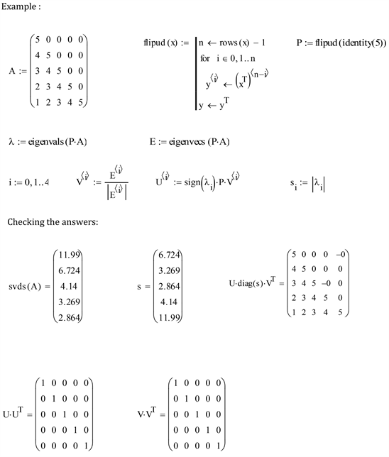
For example, if matrix A is:

$A=\left[\begin{array}{ccccc}5& 0& 0& 0& 0\\ 4& 5& 0& 0& 0\\ 3& 4& 5& 0& 0\\ 2& 3& 4& 5& 0\\ 1& 2& 3& 4& 5\end{array}\right]$

SVD of that matrix can be completed by finding U, V and D (Λ) from Equation (26) (please see Appendix for Mathcad codes).

4.2. Resolve the Example in Section 3 Using Discrete-Time SVD

In this section, the illustrative example solved in Section 3 will be resolved by the discrete-time SVD algorithm. For a discrete decomposition, the original continuous function ${\text{e}}^{-\left(t-\tau \right)}$ is first discretized as 100 discrete values, from which a Toeplitz matrix is formed and the validated SVD process presented in Equations (22) to (26) is applied to find finding U, V and D for such Toeplitz matrix. Since the SVD algorithm has been implemented into Mathcad, so the entire process is solved using that software and the detailed codes are presented below, where the embedded figure shows the discretized function $y={\text{e}}^{-t}$, which is displayed through 100 points. Figure 4 compares the first column of U with the discretized normalized function $f_1$ (Equation (18)). From that figure and Figure 2, it is confirmed that the discrete-time SVD can correctly find the output for the IRF and the first column of the SVD matrix U is the discrete solution for such problem, which can be considered as a counterpart of Equation (19) in discrete domain.

In Figure 3 and Figure 4, the $U{1}_{i1}$ is the 100 point values of the discretized function and $U{1}_{i1}/\left|U1\right|$ represents the normalized function f₁ (Equation (18))

for i from 0 to 3. ${\left(U^{\langle i\rangle }\right)}_{i1}$ is the ith column extracted from the matrix U, which

is obtained following the discrete-time SVD process presented in Figure 3 and from Equations (22) to (26).

4.3. Discussion

In this section, the discrete-time SVD is performed to solve the problem raised in Equation (2) in a discrete system. From the solution it can be seen that the presented method can accurately yield the results, which is the ith column of the SVD matrix U. The critical technique employed here is to flip the lower triangle Toeplitz matrix upside down to convert it to a Hankel matrix through a permutation matrix. Comparing to the Toeplitz matrix, which is usually used to model the IRF, the Hankel matrix is easier to be decoupled therefore making computing effort easier and more efficient. The same “flipping upside-down” technique is also applied for the continuous-time SVD (the function term $f\left(j,T-t\right)$ in Equation (1)) to simplify the solution process.

5. Continuous-Time SVD of $e^{-a\left(t-\tau \right)}$

Section 2 presents continuous-time SVD for the Green’s function ${\text{e}}^{-\left(t-\tau \right)}$. In reality, the continuous-time SVD can be used to process a wealth of IRF’s and in this section the method displayed in Section 2 is pushed one-step forward by discussing the continuous-time SVD of ${\text{e}}^{-a\left(t-\tau \right)}$.

Figure 3. Comparison between the ith column of U and the discretized normalized function f₁.

Figure 4. Mathcad codes for solution of the example using discrete-time SVD.

Back to Equation (1) and if $h\left(t,\tau \right)={\text{e}}^{-a\left(t-\tau \right)}$, where a is a real positive number, Equation (2) becomes:

${\displaystyle {\int }_0^t{\text{e}}^{a\tau }f\left(j,\tau \right)\text{d}\tau }={\text{e}}^{at}{D}_{j}f\left(j,T-t\right)$ (27)

Let $t_p=at$ and ${\tau }_p=a\tau$, then it follows that $\text{d}{\tau }_p=a\text{d}\tau$ and the integration limits become $0\le {\tau }_p\le t_p$. Substituting them back into the integral Equation (27) and we obtain:

$\frac{1}{a}{\displaystyle {\int }_0^{t_p}{\text{e}}^{{\tau }_p}f\left(j,\frac{{\tau }_p}{a}\right)\text{d}{\tau }_p}={\text{e}}^{t_p}{D}_{j}f\left(j,\frac{T\cdot a-t_p}{a}\right)$ (28)

Let $f\left(j,t\right)=\sin \left(\omega t\right)$ and Equation (28) then becomes:

${\displaystyle {\int }_0^{t_p}{\text{e}}^{{\tau }_p}\sin \left(\omega \frac{{\tau }_p}{a}\right)\text{d}{\tau }_p}=a{\text{e}}^{t_p}{D}_j\sin \left(\omega \frac{T\cdot a-t_p}{a}\right)$ (29)

Now we define ${\omega }_p=\frac{\omega }{a}$, $T{R}_p=T\ast a$ and $D_p=D\ast a$ and Equation (29) can be simplified as:

${\displaystyle {\int }_0^{t_p}{\text{e}}^{{\tau }_p}\sin \left({\omega }_p{\tau }_p\right)\text{d}{\tau }_p}={\text{e}}^{t_p}{D}_p\sin \left[{\omega }_p\left(T_p-t_p\right)\right]$ (30)

Equation (30) follows the same form as Equation (2) and then it can be solved following the same approach discussed in Section 2 (Equations (3) to (17)).

6. Conclusion

This study presented and validated continuous-time and discrete-time SVD for the impulse response function, a special kind of Green’s functions. For both the continuous-time and discrete-time SVD, the “flipping upside-down” strategy is employed to simplify the solution process. Illustrative example confirms the accuracy and efficiency of the present methods. Even though this paper mainly focuses on the SVD of the Green’s functions, it is obvious that the solution can follow a similar approach. Comparing to existing methods, one advantage of the presented method is that by using such method, the time-domain output can be directly determined from the convolution of the input with the IRF without going through Laplace and inverse Laplace transforming. Considering the diversity of impulse response functions involved in multidisciplinary engineering problems, the method presented in this study can be extensively developed for broad applications. In the future, the SVD approach can be further modified to absorb some features of Adomian decomposition method [14] [15] [16] for being used to solve more engineering problems such as Cauchy type singular integral equation [17] [18], Bagley-Torvik equation [19], Fredholm integro-differential equation [20] [21] [22].

Appendix. Verification of SVD for Toeplitz Matrices Using Mathcad

Conflicts of Interest

The authors declare no conflicts of interest regarding the publication of this paper.

References

[1]	Ramirez-Velarde, R.V., Roderus, M., Barba-Jimenez, C. and Perez-Cazares, R. (2014) A Parallel Implementation of Singular Value Decomposition for Video-on-Demand Services Design Using Principal Component Analysis. Procedia Computer Science, 29, 1876-1887. https://doi.org/10.1016/j.procs.2014.05.172
[2]	Liu, F., Yang, G., Yin, Y. and Wang, S. (2014) Singular Value Decomposition Based Minutiae Matching Method for Finger Vein Recognition. Neurocomputing, 145, 75-89. https://doi.org/10.1016/j.neucom.2014.05.069
[3]	Wan, W., Zhou, Z., Zhao, J. and Cao, F. (2015) A Novel Face Recognition Method: Using Random Weight Networks and Quasi-Singular Value Decomposition. Neurocomputing, 151, 1180-1186. https://doi.org/10.1016/j.neucom.2014.06.081
[4]	Zhang, X., Xu, Z., Jia, N., Yang, W., Feng, Q., Chen, W. and Feng, Y. (2015) Denoising of 3D Magnetic Resonance Images by Using Higher-Order Singular Value Decomposition. Medical Image Analysis, 19, 75-86. https://doi.org/10.1016/j.media.2014.08.004
[5]	Shih, Y.-T., Chien, C.-S. and Chuang, C.-Y. (2012) An Adaptive Parameterized Block-Based Singular Value Decomposition for Image De-Noising and Compression. Applied Mathematics and Computation, 218, 10370-10386. https://doi.org/10.1016/j.amc.2012.03.070
[6]	Ghazy, R.A., Amoon, M., Abdallah, H.A., El-Fishawy, N.A., Hadhoud, M.M., Dessouky, M.I., Alshebeili, S.A. and El-Samie, F.E.A. (2014) Block Based Embedding of Encrypted Watermarks Using Singular Value Decomposition. Optik, 125, 6299-6304. https://doi.org/10.1016/j.ijleo.2014.08.012
[7]	Cai, X., Sun, P., Chen, J. and Xie, L. (2014) Rapid Distributed Model Predictive Control Design Using Singular Value Decomposition for Linear Systems. Journal of Process Control, 24, 1135-1148. https://doi.org/10.1016/j.jprocont.2014.05.002
[8]	Katsaounis, T.I., Dean, A.M. and Jones, B. (2013) On Equivalence of Fractional Factorial Designs Based on Singular Value Decomposition. Journal of Statistical Planning and Inference, 143, 1950-1953. https://doi.org/10.1016/j.jspi.2013.06.013
[9]	Berenguer, L., Dufaud, T. and Tromeur-Dervout, D. (2013) Aitken’s Acceleration of the Schwarz Process Using Singular Value Decomposition for Heterogeneous 3D Groundwater Flow Problems. Computers & Fluids, 80, 320-326. https://doi.org/10.1016/j.compfluid.2012.01.026
[10]	di Dio, P.J. (2013) Thermal Stability of Water up to Super-Critical States: Application of the Singular Value Decomposition and Grund Functions. Journal of Molecular Fluids, 187, 206-217. https://doi.org/10.1016/j.molliq.2013.07.013
[11]	Abuturab, M.R. (2014) Color Information Verification System Based on Singular Value Decomposition in Gyrator Transform Domains. Optics and Lasers in Engineering, 57, 13-19. https://doi.org/10.1016/j.optlaseng.2014.01.006
[12]	Kavaklioglu, K. (2014) Robust Electricity Consumption Modeling of Turkey Using Singular Value Decomposition. International Journal of Electrical Power & Energy Systems, 54, 268-276. https://doi.org/10.1016/j.ijepes.2013.07.020
[13]	Dempsey, K.M. and Irvine, H.M. (1978) A Note on the Numerical Evaluation of Duhamel’s Integral. Earthquake Engineering Structural Dynamics, 6, 511-515. https://doi.org/10.1002/eqe.4290060507
[14]	Liu, Y.-C. (2009) Adomian Decomposition Method with Second Kind Chebyshev Polynomials. Proceedings of the Jangjeon Mathematical Society, 12, 57-67.
[15]	Liu, Y.-C. (2009) Adomian Decomposition Method with Orthogonal Polynomials: Legendre Polynomials. Mathematical and Computer Modelling, 49, 1268-1273. https://doi.org/10.1016/j.mcm.2008.06.020
[16]	Liu, Y.-C. (2012) Application of Legendre Polynomials in Adomian Pecomposition Method. Proceedings of 2012 International Conference on Computer, Electrical, and Systems Sciences, Amsterdam, 13-14 May 2012, 567-571.
[17]	Setia, A., Sharma, V. and Liu, Y.-C. (2015) Numerical Solution of Cauchy Singular Integral Equation with an Application to a Crack Problem. Neural, Parallel, and Scientific Computations, 23, 387-392.
[18]	Setia, A., Sharma, V. and Liu, Y.-C. (2017) Numerical Method of Cauchy Type Singular Integral Equation with Error Bounds. AIP Conference Proceedings, 1798, Article ID: 020141. https://doi.org/10.1063/1.4972733
[19]	Setia, A., Liu, Y.-C. and Vatsala, A.S. (2014) The Solution of the Bagley-Torvik” Equation by Using Second Kind Chebyshev Wavelet. 11th International Conference on Information Technology: New Generations, Las Vegas, 7-9 April 2014, 443-446. https://doi.org/10.1109/ITNG.2014.68
[20]	Setia, A., Liu, Y.-C. and Vatsala, A.S. (2014) Numerical Solution of Fractional Integro-Differential Equations with Nonlocal Boundary Conditions. Journal of Fractional Calculus and Applications, 5, 155-165.
[21]	Setia, A., Liu, Y.-C. and Vatsala, A.S. (2014) Solution of Linear Fractional Fredholm Integro-Differential Equation by Using Second Kind Chebyshev Wavelet. 2014 11th International Conference on Information Technology: New Generations, Las Vegas, 7-9 April 2014, 465-469. https://doi.org/10.1109/ITNG.2014.69
[22]	Liu, Y.-C. (2012) Numerical Methods for Solving Abel Integral Equation and Fredholm Integration Equation. 2012 International Conference on Computer, Electrical, and Systems Sciences, Amsterdam, 13-14 May 2012.