Fuzzy Mathematical Model for Solving Supply Chain Problem

Yi-Shian Chin¹, Hsin-Vonn Seow^1*, Lai Soon Lee^2,3, Rajprasad Kumar Rajkumar⁴

¹Nottingham University Business School, University of Nottingham Malaysia Campus, Semenyih, Malaysia.
²Laboratory Computational Statistics and Operations Research, Institute for Mathematical Research, University Putra Malasia, Serdang, Malaysia.
³Department of Mathematics, Faculty of Science, University Putra Malaysia, Serdang, Malaysia.
⁴Department of Mechanical, Materials and Manufacturing Engineering, Faculty of Engineering, University of Nottingham Malaysia Campus, Semenyih, Malaysia.

DOI: 10.4236/jcc.2018.69007                

Abstract

In a real world application supply chain, there are many elements of uncertainty such as supplier performance, market demands, product price, operation time, and shipping method which increases the difficulty for manufacturers to quickly respond in order to fulfil the customer requirements. In this paper, the authors developed a fuzzy mathematical model to integrate different operational functions with the aim to provide satisfy decisions to help decision maker resolve production problem for all functions simultaneously. A triangular fuzzy number or possibilistic distribution represents all the uncertainty parameters. A comparison between a fuzzy model, a possibilistic model and a deterministic model is presented in this paper in order to distinguish the effectiveness of model in dealing the uncertain nature of supply chain. The proposed models performance is evaluated based on the operational aspect and computational aspect. The fuzzy model and the possibilistic model are expected to be more preferable to respond to the dynamic changes of the supply change network compared to the deterministic model. The developed fuzzy model seems to be more flexible in undertaking the lack of information or imprecise data of a variable in real situation whereas possibilistic model is more practical in solving an existing systems problem that has available data provided.

Keywords

Supply Chain, Fuzzy Model, Possibilistic Model, Undertainty, Triangular Fuzzy Number

1. Introduction

In today’s global marketplace, individual enterprise is no longer sought after for individual achievement. In order to secure their business under rigorous market pressure and challenges for a long-term perspective, they tend to integrate themselves as part of the supply chain to propel their business. As the internet and information technology grow rapidly, the flow of information among different functions is the main key to drive supply chain performance. [1] shares the five main supply chain practices that will equip a business to stay competitive and improve its organizational performance. These are supplier partnership, customer relationship, quality of information sharing, level of information sharing and postponement. In other words, the truly integrated and strong relationship formed among supply chain members is an essential prerequisite to succeed in the global market.

The attention on the development of the concept for supply chain management has gradually drawn the attention from academicians, business/industry managers, and consultants. The concept has been evaluated, practiced, examined and proven to be able to address various supply chain issues and influence the firm’s performance [1] [2] [3] . A supply chain model plays a significant role in supply chain management (SCM) for reducing the operational costs, reducing cycle time, and improving order-fulfilment rate and customer satisfaction level. This approach is proven and verified to be able to increase supply chain efficiency and delivers extra value to customers.

A supply chain (SC) is a dynamic network that consists of a high degree of uncertainty that generates from the flow of material and information, and passes through different operational functions in order to deliver goods to the end user. In general, a whole supply chain is triggered by demands from downstream sites (customers) and upstream sites (procurement, production, and distribution) which are cooperating and coordinating to transform raw materials into finished products and deliver it to customers [4] . The problem of this study is to consider a supply chain that consists of all functions and the need to meet the customers’ demand on time; with possible uncertainties occurring from all parties in the supply chain network. Much research has been carried out work to address the supply chain problem by contemplating different operational functions rather than to integrate all functions due to the complexity of a supply chain. Thus, there is little work on an integrated manner to solving the resources’ planning in this supply chain problem.

The SC problems can be disintegrated according to the time horizon and making a right decision will enable one to stabilize the SC process performance for a certain period [5] . The decision model for the supply chain planning is categorized into three levels, which are strategic, tactical, and operational [6] . A strategic model is recognized as a long term planning model that has impact on the supply chain performance for five to ten years. Most of the strategy planning consists of supply chain design and configuration, supply strategy, location-allocation problem, plant sizing, product selection, capacity expansion and distribution channel design [7] . A tactical model is considered as a mid-term planning model and mostly applied in optimizing SC process performance by utilizing available resources such as supplier, inventory, distribution center and transportation. This mid-term model is use for one to two years planning efforts. An operational model is characterized as a short-term planning model and focuses on schedule details such as lot size, day-to-day processing variations, cancellation or top up orders, vehicle route, and an assigned load [5] . In this study, a tactical model will be designed and developed for the supply chain planning problems dealing with uncertainty which has not been researched much upon.

2. Literature Review

In the 90s and before the fuzzy set theory was introduced, operation management was leaning towards reducing the complex real world problems with attributes of precise mathematical modeling and this approach became one of the most important fields in science and engineering at that time. However, researchers realized that a precise mathematical model is not achievable under “real-world” supply chain situations. Thus, they started to employ the concept and techniques of probability theory to deal with this real-world uncertainty situation. Fuzzy set theory which was first introduced by [8] started being used to define the imprecision of data based on degree of fitness rather than random variables [9] .

In Operations Research, fuzzy set theory has been applied techniques of linear and nonlinear programming, dynamic programming, production resource planning, queueing theory, multi-objective decision-making, to name a few applications [2] [9] . In 1978, [10] presented another theory that relates to the fuzzy sets and named it as Possibilistic Theory. He demonstrated under “information provided” situation, most of the decision-making is based on the possibilistic nature rather than probability. [11] explained that probability describes whether the event occurs and to what degree of it occurs is fuzzy. Fuzzy set theory is a theory of graded concept (degree of a matter) and is not focused on a chance the event will occur; this is the difference between concept randomness and fuzziness [9] . Possibilistic Theory explains how likely of the event may happen. Possibility theory is treats as alternative of probability theory to deal with the uncertain situation. This shows that the probability model has its limitations in modelling all possible problems of incompleteness.

Fuzzy modeling approach is widely used in solving the problems in aggregate planning, manufacturing resource planning, transportation planning, inventory management, and supply chain planning [12] . The fuzzy set theory has been applied to different problems related to the supply chain planning, such as the following:

1) Aggregate planning

[13] proposed a model based on set theory for solving the aggregate production planning (APP) problem which identify demand and process uncertainty. Trapezoidal fuzzy number is used to present the fuzzy parameters in the model. They state that traditional linear programming is not the best choice for predicting medium and long-term planning horizon due to the fluctuation of market demands and inconsistency of production parameters in real situation. They proposed a fuzzy linear programming approach that is more adequate and realistic approach to use for solving the production planning problem through continuous modeling problem according to the available information.

2) Manufacturing resource planning

[14] compared the traditional LP with deterministic coefficient with a fuzzy linear programming model in determining the production-planning schedule for fresh tomato packing in Ruskin, Florida. This study showed the fuzzy linear programming approach is more practical and characterized the real-life tomato-packing situation by relaxing some resource restriction. Results showed that the average operation cost using the fuzzy modeling method is 10 times less than traditional linear programming and the service satisfaction level increased as well. [15] used possibilistic theory combined with [16] ’s fuzzy programming method to obtain a compromise solution to minimize the production operation cost and decision satisfactory information. This approach was implemented in production for resource planning in dealing with assemble-to-order environment under demand uncertainty situation. The solution helped in determining the safety stock level and to decide the number of key machined used for reducing the capital waste. This paper results showed that this approach was competent in the decision making process when dealing with imprecise data. [17] applied a similar approach as [15] in solving a real industry aggregate production planning (APP) problem in their research to help determine the 18-month production resource-planning. The solution could be improved through iteratively modifying the possibilistic distirbution. [17] demonstrated that a compromise solution for APP can be obtained with the overall satisfaction result guidance in the modelling process.

3) SC inventory management

[18] aimed at integrating the SC model with simulation control to determine the inventory’s stock level and order quantity in a finite time horizon, to minimize the supply chain cost, with an acceptable delivery performance. The uncertainties considered in the fuzzy model are external supplier late delivery and fluctuation of customer demand. The SC model was developed to deal for the uncertainty elements and determine the inventory’s order-up-to stock level; whereas the SC simulator was used to evaluate the decision made by the SC fuzzy model. [19] extends his research work with a proposed simulation tool named SCSIM to do analysis and evaluate the dynamic behavior of a series of supply chain under uncertain environment to enhance the decision making.

4) Transportation planning

[20] proposed a fuzzy mathematical programming model to minimize overall supply chain cost through identifying the allocation of orders to depots, arrangement of sending and returning of vehicles to depots. This model is built with consideration with multiple depots, multiple vehicles, multiple products, multiple customers and with different periods. A two-ranking function is used to solve planning problems and a regression model is developed to analyze the applied fuzzy ranking method. Results expressed the flexibility of fuzzy modeling in representing a real life environment.

[21] optimized the supply chain procurement transportation operational planning (SCPTOP) problem using fuzzy multi-objective integer linear programming model (FMOLP). This solution in a real automobile industry sector with integration with the automobile assembler, a first tier supplier and second-tier supplier was used in solving the procurement and transportation-planning problem simultaneously. This study helps decision-makers convert the manual decision procedure into an automatic mode, which provides a better result in controlling their total stock level, and benefits each supply chain party.

5) Supply chain planning

[22] designed a supply chain scheduling model to solve multiproduct, multistage, and multi-period under uncertain demands and product price situation. This research study developed a mixed integer nonlinear programming (MINLP) model to simultaneously optimize multiple objectives such as achieving fair profit distribution among supply chain partners, optimized safe inventory levels, maximizing customer service levels, maximum robustness to demand uncertainties and guaranteed acceptance of product price. This study demonstrated that a fuzzy modelling approach is able to provide a solution for solving multiple conflicts that exist in a supply chain while under uncertainty. This research work is then extended to determine the location of the warehouse and distribution centers based on a consideration of total cost, local incentives and transport time [23] . [24] combined a fuzzy model and PERT to compute the total time of an entire supply chain system (supplier, manufacturer, distribution and retail). This research consists of a multi-stage and multi-echelon supply chain system. A triangular fuzzy number is used to present various uncertainties in operation time. The proposed model was able to simulate and provide the shortest SC completion time path in fulfilling the customer’s request. However, if the simulation result showed that the customer demand was not completed within the requested time, the enterprise would respond and adjust the promised-delivery possibility (PDP) value to increase the order-fulfillment ability. This approach indirectly increases the efficiency of the entire system and the competitiveness of supply chain. [25] proposed a fuzzy model with multi-product, multi-echelon, and multi-period to calculate the lower and upper bound of minimum total supply chain operation cost with optimization on the arrangement of the operation plan. The model developed was based on α-cut representation and Zadeh’s extension principle; fuzzy parameters are expressed by triangular and trapezoidal fuzzy number. More recently, [26] reported an investigation regarding the benefit of using fuzzy set theory to model and solve supply chain problems in the manufacturing industry. This model has been tested with the real data obtained from a real-world automobile supply chain by using CPLEX software. The research result expresses that fuzzy modeling is clearly superior to deterministic model in handling the real situations especially when there are pre-existing imprecise information. [27] extends this research, which includes a supply chain global satisfaction degree by considering the aspect of service level, inventory cost, planning nervousness (period and quantity) and overall cost. [28] revealed that the design of a supply chain has more advantages when dealing with supply uncertainty for a multi-stage and multi-echelon supply chain network. They expressed that supply chain centralization is always a suitable strategy under high or low risk supply uncertainty and it able to fulfill market demand with lowest price.

[29] proposed to apply the possibilistic approach in solving the water quality management planning problem and this solution help in solving economic and environmental factor simultaneously. An inexact agricultural water quality management (IAWQM) model is developed to consider the agricultural activities can be generated under restriction of water quality and quantity variable in order to maximize the agricultural income. The result provided a schematic decision in identify the cropping area, fertilizer applied and livestock husbandry size, incorporating water management knowledge. [30] extended [15] research work by applying a similar possibilistic approach into the supply chain modelling to solve for multi-product and multi-period manufacturing and distribution planning decision (MDPD) in the real SC situation. In this research, the effectiveness of a possibilistic model and deterministic model is compare in solving the SC planning problem under the uncertainty. Research result presets that the proposed possibilistic model solution is more efficient and practical when practiced in the real world MDPD. [31] proposed a possibilistic linear programming model to solve for supply chain problems in the bus-manufacturing company. 11 experiments have been designed, with a sensitivity analysis test to validate the consistency of the model. The solution was able to provide the manager with information and guidance in preparing their strategy for in-house resources planning.

A lot of supply chain research focus on a specific area such as supplier selection, transportation planning, facility location, manufacturing resources planning, and aggregate planning. Very few address the supply chain problem integrating all functions together. The authors try to address this problem through the development of a mathematical model that integrates procurement, production, and distribution decision. In this study, fuzzy set theory and possibilistic theory are applied instead of using probabilistic distribution, which can be derived from historical data. This is because in a real-world supply chain, not all the relevant variables has existing data and imprecise of data will directly affect the result. Thus, these two theories are best used to represent the characteristics of imprecise data, lack of information or a new design product forecast for those uncertainties parameters in the model. This study proposes a multi-stage, single product, multi-echelon and multi-period supply chain network to investigate the benefit of the fuzzy linear programming (FLP) model and possibilistic linear programming (PLP) in dealing with demand uncertainty, process uncertainty and supply uncertainty issues.

This study focuses on optimizing the supply chain resources’ planning under demand, supply and process uncertainties with using mixed-integer linear programming method. A fuzzy mathematic model is developed integrating different functions of the supply chain with target to minimize the operational cost using an optimal planning solution. The objectives of this study are:

1) To model a supply chain problem that deals with procurement, production, and distribution planning under uncertainty.

2) To develop a mathematic model to include uncertainties from supplier, process and demand, where these parameters are represented by a triangular fuzzy number.

3) To provide solutions to resolve decision-making problems for different operational functions simultaneously with a developed model.

4) To investigate the benefits and effectiveness of fuzzy set theory in FLP and PLP in modeling and solving supply chain problem.

3. Case Description

This study describes the multi-stage, multi-echelon, multi-time period, single product and single objective fuzzy possibilistic model which incorporates three types of uncertainty. The types of uncertainty involved in this model are demand uncertainty, process uncertainty and supplier uncertainty. This supply chain system consists of four echelons which are supplier, production plant, distribution and customer as shown in Figure 1.

This model is assumes a single product is manufactured at one time period, and each product is made by two types of raw material. The objective of a fuzzy linear programming approach is proposed in this paper is aimed to minimize operation cost while providing a systematic framework which is able to integrate all fuzzy variables in the supply chain model under uncertainty. This approach is also considers the decision makers’ satisfaction and enable them adjust the fuzzy parameters in order to obtain a satisfy solution.

The following are the assumptions made for modelling the supply chain model:

1) Each customer order is independent. Backorder demand is considered in this supply chain and backorder demand must be fulfilled in the next time period.

2) All demands must be fulfilled at the end of the planning horizon and no backorder demand is allowed in the end of planning horizon.

3) A backlog order’s maximum unit is limited at 50 for each time period which is approximately 10% of the order in each time period.

Figure 1. Supply chain link: research region.

4) All the fuzzy parameters are represented using a triangular membership function.

5) No safety stock is considered in the production plant and distribution center’s inventory.

Many parameters are introduced in this supply chain model which includes general data, decision variables and fuzzy variables. In this formulation, a waving symbol (^~) is used to represent a fuzzy variable. Dimension explains the echelons [supplier(s), plant (p), distribution center(r) and customer(c)] involved for each variables in the mathematic model (Table 1).

3.1. Fuzzy and Fuzzy Possibilistic Linear Programming Model

3.1.1. Objective Function

In this study, the proposed linear programming objective is to minimize the overall operation cost though optimized arrangement of the operation resources. The cost coefficients consider in multi-stage, multi-echelon and multi-time period model are raw material cost, production cost, inventory cost, transportation cost and demand backlog cost. The following is the fuzzy objective function for minimize the operation cost:

$\begin{array}{c}\tilde{z}=\min \cdot [{\displaystyle \underset{t=0}{\overset{T}{\sum }}{\displaystyle \underset{s=0}{\overset{S}{\sum }}{\displaystyle \underset{f=0}{\overset{F}{\sum }}RM{C}_{fs}\cdot B{Q}_{fst}}}}+{\displaystyle \underset{t=0}{\overset{T}{\sum }}{\displaystyle \underset{p=0}{\overset{P}{\sum }}{\displaystyle \underset{g=0}{\overset{G}{\sum }}{\widetilde{PC}}_{gpt}\cdot P{Q}_{gpt}}}}\\ +{\displaystyle \underset{t=0}{\overset{T}{\sum }}{\displaystyle \underset{p=0}{\overset{P}{\sum }}{\displaystyle \underset{f=0}{\overset{F}{\sum }}IL{R}_{fpt}\cdot {\widetilde{IC}}_{pt}}}}+{\displaystyle \underset{t=0}{\overset{T}{\sum }}{\displaystyle \underset{r=0}{\overset{R}{\sum }}{\displaystyle \underset{g=0}{\overset{G}{\sum }}I{R}_{grt}\cdot {\widetilde{HC}}_{grt}}}}\\ +{\displaystyle \underset{t=0}{\overset{T}{\sum }}{\displaystyle \underset{s=0}{\overset{S}{\sum }}{\displaystyle \underset{p=0}{\overset{P}{\sum }}{\displaystyle \underset{f=0}{\overset{F}{\sum }}{\widetilde{TC}}_{fpst}\cdot B{Q}_{fpst}}}}}+{\displaystyle \underset{t=0}{\overset{T}{\sum }}{\displaystyle \underset{p=0}{\overset{P}{\sum }}{\displaystyle \underset{r=0}{\overset{R}{\sum }}{\displaystyle \underset{g=0}{\overset{G}{\sum }}{\widetilde{TC}}_{gprt}\cdot P{R}_{gprt}}}}}\\ +{\displaystyle \underset{t=0}{\overset{T}{\sum }}{\displaystyle \underset{r=0}{\overset{R}{\sum }}{\displaystyle \underset{c=0}{\overset{C}{\sum }}{\displaystyle \underset{g=0}{\overset{G}{\sum }}{\widetilde{TC}}_{cgrt}\cdot P{E}_{cgrt}}}}}+{\displaystyle \underset{t=0}{\overset{T}{\sum }}{\displaystyle \underset{g=0}{\overset{G}{\sum }}{\displaystyle \underset{c=0}{\overset{C}{\sum }}D{B}_{gct}\cdot {\widetilde{DBC}}_{ct}}}}]\end{array}$ (1)

1) The total raw material cost:

The unit of raw material cost multiplied by the total of purchase amount

(a) (b)

Table 1. Nomenclature for supply chain model.

brought into production plant is the total raw material cost on period t.

$\underset{t=0}{\overset{T}{{\displaystyle \sum }}}\underset{s=0}{\overset{S}{{\displaystyle \sum }}}\underset{f=0}{\overset{F}{{\displaystyle \sum }}}RM{C}_{fs}\cdot B{Q}_{fst}$ (2)

2) The total production cost:

Total amount of product, g manufactured in plant p multiplied by the unit product cost is equal to the production cost on period t.

$\underset{t=0}{\overset{T}{{\displaystyle \sum }}}\underset{p=0}{\overset{P}{{\displaystyle \sum }}}\underset{p=0}{\overset{G}{{\displaystyle \sum }}}{\widetilde{PC}}_{gpt}\cdot P{Q}_{gpt}$ (3)

3) The total inventory cost:

a) Plant’s inventory cost:

This model assumes that each plant p has its own inventory for storing the finished goods and remaining raw material left from the previous period t. However, this inventory has its capacity and inventory holding will be charged. Inventory in the production plant p includes raw material and finished goods.

$\begin{array}{l}{{\displaystyle \sum }}^{\text{}}\text{Plant Inventory cost}\\ ={{\displaystyle \sum }}^{\text{}}\text{Raw material inventory cost}+{{\displaystyle \sum }}^{\text{}}\text{Finished product inventory cost}\end{array}$

For the inventory level of raw material f at the plant, p in time period t, the balance equation can be written as follow:

Inventory in the end of the period t = inventory level of period t − 1 + received raw material f shipment from supplier s in time period t ? total material used for manufacture product g in time period t.

So for time period t = 1:

$IL{R}_{fpt}=\underset{s=0}{\overset{S}{{\displaystyle \sum }}}B{Q}_{fpst}-\left(\underset{g=0}{\overset{G}{{\displaystyle \sum }}}BO{M}_{fg}\cdot \underset{g=0}{\overset{G}{{\displaystyle \sum }}}P{Q}_{gpt}\right),\forall f,p,t$

For time period t > 1:

$IL{R}_{fpt}=IL{R}_{fp\left(t-1\right)}+\underset{s=0}{\overset{S}{{\displaystyle \sum }}}B{Q}_{fpst}-\left(\underset{g=0}{\overset{G}{{\displaystyle \sum }}}BO{M}_{fg}\cdot \underset{g=0}{\overset{G}{{\displaystyle \sum }}}P{Q}_{gpt}\right),\forall f,p,t$ (4)

For the inventory level of finished product g at the plant p in time period t, the balance equation can be written as follows:

Inventory in the end of the period t = inventory level of period t − 1 + total manufacturer product g manufactured in plant p in time period t − total quantity of finished product g deliver from plant p to distribution center r in time period t.

For time period t = 1:

$IL{G}_{gpt}=P{Q}_{gpt}-\underset{r=0}{\overset{R}{{\displaystyle \sum }}}P{R}_{gprt},\forall g,p,t$

For time period t > 1:

$IL{G}_{gpt}=IL{G}_{gp\left(t-1\right)}+P{Q}_{gpt}-\underset{r=0}{\overset{R}{{\displaystyle \sum }}}P{R}_{gprt},\forall g,p,t$ (5)

Thus, the summation of the inventory cost in plant p in time period t can be written as follow:

$\begin{array}{l}{{\displaystyle \sum }}^{\text{}}\text{Plant Inventory cost}\\ ={{\displaystyle \sum }}^{\text{}}\text{Raw material inventory cost}+{{\displaystyle \sum }}^{\text{}}\text{Finished product inventory cost}\\ =\left(\underset{t=0}{\overset{T}{{\displaystyle \sum }}}\underset{p=0}{\overset{P}{{\displaystyle \sum }}}\underset{f=0}{\overset{F}{{\displaystyle \sum }}}IL{R}_{fpt}\cdot {\widetilde{IC}}_{pt}\right)+\left(\underset{t=0}{\overset{T}{{\displaystyle \sum }}}\underset{p=0}{\overset{P}{{\displaystyle \sum }}}\underset{g=0}{\overset{G}{{\displaystyle \sum }}}IL{G}_{gpt}\cdot {\widetilde{IC}}_{pt}\right)\end{array}$ (6)

b) Distribution center’s inventory cost:

Distribution center r also has its inventory space to keep the finished product, g before shipping to customer c in time period t. The balance equation can be written as follows:

Inventory in the end of the period t = inventory level of period t − 1 + receive finish product g from plant p in time period t − total quantity of product g deliver to customer c from distribution center r in time period t.

For time period t = 1:

$I{R}_{grt}=\underset{p=0}{\overset{P}{{\displaystyle \sum }}}P{R}_{grpt}-\underset{c=0}{\overset{C}{{\displaystyle \sum }}}P{E}_{cgrt},\forall g,r,t$

For time period t > 1:

$I{R}_{grt}=I{R}_{gr\left(t-1\right)}+\underset{p=0}{\overset{P}{{\displaystyle \sum }}}P{R}_{gprt}-\underset{c=0}{\overset{C}{{\displaystyle \sum }}}P{E}_{cgrt},\forall g,r,t$ (7)

Thus, the sum of the distribution center’s (DC) inventory cost consumption can be written as follow:

$\begin{array}{l}{{\displaystyle \sum }}^{\text{}}\text{Distribution center inventory cost}\\ ={{\displaystyle \sum }}^{\text{}}\text{DC}’\text{sinventory level}\cdot \text{inventory holding cost}\\ =\underset{t=0}{\overset{T}{{\displaystyle \sum }}}\underset{r=0}{\overset{R}{{\displaystyle \sum }}}\underset{g=0}{\overset{G}{{\displaystyle \sum }}}I{R}_{grt}\cdot {\widetilde{HC}}_{grt}\end{array}$ (8)

4) The total transportation cost:

Total transportation cost is divide into 3 stages, it includes:

a) sum of the raw material’s delivery cost from supplier, s to production plant, p in time period t;

b) shipment cost to delivery product from plant, p to distribution center, r in time period t;

c) shipment cost for ready stock delivery from distribution center, r to customer, c site in time period t.

The balance equation can be written as follow:

Transportation cost in the end of the period t = shipping cost for deliver raw material f from suppliers to plant p in time period t + deliver the finish product g from plant p to distribution center in time period t + total quantity of product g deliver to customer c from distribution center r in time period t.

$\begin{array}{l}{{\displaystyle \sum }}^{\text{}}\text{Transportationcost}\\ ={{\displaystyle \sum }}^{\text{}}\text{Trans}\text{.supplier\_plant}+{{\displaystyle \sum }}^{\text{}}\text{Trans}\text{.plant\_DC}+{{\displaystyle \sum }}^{\text{}}\text{TransDC\_cust}\end{array}$

The total transport cost from supplier, s to production plant, p for raw material, f shipment in time period t:

$\underset{t=0}{\overset{T}{{\displaystyle \sum }}}\underset{p=0}{\overset{P}{{\displaystyle \sum }}}\underset{r=0}{\overset{R}{{\displaystyle \sum }}}\underset{g=0}{\overset{G}{{\displaystyle \sum }}}{\widetilde{TC}}_{fpst}\cdot B{Q}_{fpst}$ (9)

The total transport cost from production plant, p to distribution center, r for product, g shipment in time period t:

$\underset{t=0}{\overset{T}{{\displaystyle \sum }}}\underset{p=0}{\overset{P}{{\displaystyle \sum }}}\underset{r=0}{\overset{R}{{\displaystyle \sum }}}\underset{g=0}{\overset{G}{{\displaystyle \sum }}}{\widetilde{TC}}_{gprt}\cdot P{R}_{gprt}$ (10)

The total transport cost from distribution center, r to customer, c for product, g shipment in time period t:

$\underset{t=0}{\overset{T}{{\displaystyle \sum }}}\underset{r=0}{\overset{R}{{\displaystyle \sum }}}\underset{c=0}{\overset{C}{{\displaystyle \sum }}}\underset{g=0}{\overset{G}{{\displaystyle \sum }}}{\widetilde{TC}}_{cgrt}\cdot P{E}_{cgrt}$ (11)

5) Demand backlog cost:

If output of production plant is unable to meet the demand target as per customer request, the shortage unit is considered as demand backlog and penalty will be charge for the delay in shipment. The balance equation of demand backlog on period t can be written as follow:

Demand backlog of the period t = demand backlog level of period t − 1 + demand request by customer c in time period t − total quantity of product g deliver to customer c from distribution center r in time period t.

For time period t = 1:

$D{B}_{gct}=D_{cgt}-\underset{r=0}{\overset{R}{{\displaystyle \sum }}}P{E}_{cgrt},\forall g,c,t$

For time period t > 1:

$D{B}_{gct}=D{B}_{gc\left(t-1\right)}+D_{cgt}-\underset{r=0}{\overset{R}{{\displaystyle \sum }}}P{E}_{cgrt},\forall g,c,t$ (12)

The demand backlog cost multiplied by the total shortage quantity is the demand backlog consumption.

$\underset{t=0}{\overset{T}{{\displaystyle \sum }}}\underset{g=0}{\overset{G}{{\displaystyle \sum }}}\underset{c=0}{\overset{C}{{\displaystyle \sum }}}D{B}_{gct}\cdot {\widetilde{DBC}}_{ct}$ (13)

3.1.2. Constraints

1) Supplier constraint

The total amount of purchase raw material f from each supplier, s should not greater than maximum procurement capacity.

$B{Q}_{sft}\le {\widetilde{MBC}}_{sf},\forall s,f,t$ (14)

2) Demand constraint

Assumes that the total amount of product g shipped from distribution center, r to each customer, c is referred as customer demand. The amount of product deliver to customer c is as per order requested.

${\tilde{D}}_{cgt}=\underset{r=0}{\overset{R=0}{{\displaystyle \sum }}}P{E}_{cgrt},\forall c,g,t$ (15)

3) Inventory constraint

Inventory stock level for raw material, f and finish product, g in plant, p cannot exceed the maximum inventory capacity level in time period t. Distribution center’s inventory also applies the same rule.

a) Plant’s inventory constraint

Let IL be defined as the plant’s inventory level which use for stores the raw material, f and finished product, g in time period t.

$I{L}_{pt}=\underset{f=0}{\overset{F}{{\displaystyle \sum }}}IL{R}_{fpt}+\underset{g=0}{\overset{G}{{\displaystyle \sum }}}IL{G}_{gpt},\forall p,t$ (16)

The plant inventory level, IL is controlled not to exceed the plant’s maximum inventory capacity in time period t.

$I{L}_{pt}\le MI{C}_P,\forall p,t$ (17)

b) Retailer’s inventory constraint:

The distribution inventory level, IR is controlled not to exceed the distribution center’s, r maximum inventory capacity in time period t.

$I{R}_{grt}\le MR{C}_{gr},\forall g,r,t$ (18)

4) Production constraint

The quantity of product, g manufactured in plant, p is controlled to not to exceed the maximum production capacity.

$P{Q}_{gpt}\cdot {\widetilde{PT}}_{gp}\le {\widetilde{MPC}}_{gp},\forall g,p,t$ (19)

5) Transportation constraint

The product, g ships out quantity from plant, p to distribution center, r should not exceed the limit of transportation capacity. It applies the same rule for the transportation from distribution center, r to customer zone, c.

$P{Q}_{gprt}\le {\widetilde{MTC}}_{gpr},\forall g,p,r,t$ (20)

$P{R}_{grct}\le {\widetilde{MTC}}_{grc},\forall g,r,c,t$ (21)

6) Demand backlog constraint

The total of finished product g shipped to customer c is always less than the total amount of demand on time t plus the demand backlog of previous period, t − 1.

$P{E}_{cgt}\le D{B}_{gt-1}+D_{cgt},\forall c,g,t$ (22)

3.2. Strategy to Convert Fuzzy Objective into Equivalent Auxiliary Crisp Linear Programming for FLP Model

In order to transform the fuzzy mixed integer linear programming (FMILP) into an equivalent auxiliary crisp MILP model a special treatment need to be perform for those uncertainty parameter in the model. The uncertainty elements in this model are supplier, process operation and demand. These uncertainties are labelled as fuzzy coefficients existing in the objective function and constraint in the model. In order to address the uncertainty parameters for FMILP, the approach of representation theorem and technological coefficient proposed by [32] is applied in this study.

The transformation from fuzzy mixed integer linear programming (FMILP) to auxiliary a parametric integer linear programming is written as following:

Objective function:

$\max cx$

Subject to: $f\left(\underset{j=1}{\overset{n}{{\displaystyle \sum }}}{\tilde{A}}_{ij}{x}_j\right)\le f\left({\tilde{b}}_i+{\tilde{t}}_i\left(1-\alpha \right)\right),i\in M,$

(23)

(from [32] )

Explanation of parameters: $c$ = fuzzy coefficient of objective function; = fuzzy coefficient of ith constraint; = fuzzy resources of ith constraint; = fuzzy number in the maximum violation allowed of the ith constraint; = degree of membership function, within the range of [0, 1].

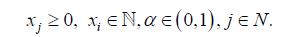
To simplify, a linear membership function, the triangular fuzzy number is proposed to be used to represent all the fuzzy parameter and the first index of Yager is applied into the auxiliary parametric crisp model. The Triangular fuzzy number is denoted as 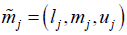which represents low, medium and high value of the function. To deal with the imprecise coefficients and fuzzy inequalities in the constraints, linear ranking function and Yager’s index first type theory is applied [32] [33] :

Below is the Yager’s index formulation:

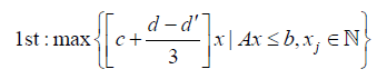(24)

where c is the fuzzy parameter exist in the objective function and d’ and d is lateral margin of the triangular fuzzy number center point, m.

Yager’s theory considers all the fuzzy subsets as normal and convex, which is represented as ${\tilde{u}}_i,i\in \mathbb{N}=\left\{1,2,\cdots ,n\right\}$ . This study applies linear ranking function and considers triangular fuzzy numbers, thus first Yager’s index is proposed to apply into crisp equivalent linear programming [26] [32] [34] . Figure 2 and Figure 3 present the triangular fuzzy number and explains the method to obtain the lateral margin, ${d^{\prime }}_j$ and d value that use in Yager’s first index.

By applying Yager’s first index ((Equations (3)-(24))) into Herrere and Verdegay’s theorem and technological coefficient, the crisp equivalent linear programming model is derived as follows:

$\min z=\underset{j=1}{\overset{n}{{\displaystyle \sum }}}\left(c_j+\frac{d_{cj}-{d^{\prime }}_{cj}}{3}\right)\cdot x_j$

Subject to: $\begin{array}{l}\underset{j=1}{\overset{n}{{\displaystyle \sum }}}\left(A_{ij}+\frac{d_{aij}-{d^{\prime }}_{aij}}{3}\right)\cdot x_{ij}\\ \le \left(b_i+\frac{d_{bi}-{d^{\prime }}_{bi}}{3}\right)+\left(t_i+\frac{d_{ti}-{d^{\prime }}_{ti}}{3}\right)\cdot \left(1-\alpha \right),i\in M,j\in \mathbb{N},\alpha \in \left[0,1\right]\end{array}$ (25)

$\begin{array}{c}z=\min \cdot [\underset{t=0}{\overset{T}{{\displaystyle \sum }}}\underset{s=0}{\overset{S}{{\displaystyle \sum }}}\underset{f=0}{\overset{F}{{\displaystyle \sum }}}RM{C}_{fs}\cdot B{Q}_{fst}+\underset{t=0}{\overset{T}{{\displaystyle \sum }}}\underset{p=0}{\overset{P}{{\displaystyle \sum }}}\underset{g=0}{\overset{G}{{\displaystyle \sum }}}\left(P{C}_{gpt}+\frac{d_{PC}-{d^{\prime }}_{PC}}{3}\right)\cdot P{Q}_{gpt}\\ +\underset{t=0}{\overset{T}{{\displaystyle \sum }}}\underset{p=0}{\overset{P}{{\displaystyle \sum }}}\underset{f=0}{\overset{F}{{\displaystyle \sum }}}IL{R}_{fpt}\cdot \left(I{C}_{pt}+\frac{d_{IC}-{d^{\prime }}_{IC}}{3}\right)+\underset{t=0}{\overset{T}{{\displaystyle \sum }}}\underset{p=0}{\overset{P}{{\displaystyle \sum }}}\underset{g=0}{\overset{G}{{\displaystyle \sum }}}IL{G}_{gpt}\cdot \left(I{C}_{pt}+\frac{d_{IC}-{d^{\prime }}_{IC}}{3}\right)\\ +\underset{t=0}{\overset{T}{{\displaystyle \sum }}}\underset{r=0}{\overset{R}{{\displaystyle \sum }}}\underset{g=0}{\overset{G}{{\displaystyle \sum }}}I{R}_{grt}\cdot \left(H{C}_{grt}+\frac{d_{HC}-{d^{\prime }}_{HC}}{3}\right)+\underset{t=0}{\overset{T}{{\displaystyle \sum }}}\underset{s=0}{\overset{S}{{\displaystyle \sum }}}\underset{p=0}{\overset{P}{{\displaystyle \sum }}}\underset{f=0}{\overset{F}{{\displaystyle \sum }}}B{Q}_{fpst}\cdot \left(T{C}_{fpst}+\frac{d_{TC}-{d^{\prime }}_{TC}}{3}\right)\\ +\underset{t=0}{\overset{T}{{\displaystyle \sum }}}\underset{p=0}{\overset{P}{{\displaystyle \sum }}}\underset{r=0}{\overset{R}{{\displaystyle \sum }}}\underset{g=0}{\overset{G}{{\displaystyle \sum }}}P{R}_{gprt}\cdot \left(T{C}_{gprt}+\frac{d_{TC}-{d^{\prime }}_{TC}}{3}\right)\\ +\underset{t=0}{\overset{T}{{\displaystyle \sum }}}\underset{r=0}{\overset{R}{{\displaystyle \sum }}}\underset{c=0}{\overset{C}{{\displaystyle \sum }}}\underset{g=0}{\overset{G}{{\displaystyle \sum }}}P{E}_{cgrt}\cdot \left(T{C}_{cgrt}+\frac{d_{TC}-{d^{\prime }}_{TC}}{3}\right)\\ +\underset{t=0}{\overset{T}{{\displaystyle \sum }}}\underset{g=0}{\overset{G}{{\displaystyle \sum }}}\underset{c=0}{\overset{C}{{\displaystyle \sum }}}D{B}_{gct}\cdot \left(DB{C}_{ct}+\frac{d_{DBC}-{d^{\prime }}_{DBC}}{3}\right)]\end{array}$ (26)

Special Treatment of the Imprecise Constraint for Fuzzy Linear Programing Model

After implement a special treatment on the fuzzy constraint, the equation of the model is represent as following:

$\left(D_{cgt}+\frac{d_D-{d^{\prime }}_D}{3}\right)=\underset{r=0}{\overset{R=0}{{\displaystyle \sum }}}P{E}_{cgrt},\forall c,g,t$ (27)

$B{Q}_{sft}\le \left(MB{C}_{sf}+\frac{d_{MBC}-{d^{\prime }}_{MBC}}{3}\right)+\left(t_1+\frac{d_{t_1}-{d^{\prime }}_{t_1}}{3}\right)\cdot \left(1-\alpha \right),\forall s,f,t$ (28)

For t = 1:

$IL{R}_{fpt}=\underset{s=0}{\overset{S}{{\displaystyle \sum }}}B{Q}_{fpst}-\left(\underset{g=0}{\overset{G}{{\displaystyle \sum }}}BO{M}_{fg}\cdot \underset{g=0}{\overset{G}{{\displaystyle \sum }}}P{Q}_{gpt}\right),\forall f,p,t$

For t > 1:

$IL{R}_{fpt}=IL{R}_{fp\left(t-1\right)}+\underset{s=0}{\overset{S}{{\displaystyle \sum }}}B{Q}_{fpst}-\left(\underset{g=0}{\overset{G}{{\displaystyle \sum }}}BO{M}_{fg}\cdot \underset{g=0}{\overset{G}{{\displaystyle \sum }}}P{Q}_{gpt}\right),\forall f,p,t$ (29)

Figure 2. Triangular fuzzy number.

Figure 3. Triangular membership function (TFN).

For t = 1:

$IL{G}_{gpt}=P{Q}_{gpt}-\underset{r=0}{\overset{R}{{\displaystyle \sum }}}P{R}_{gprt},\forall g,p,t$

For t > 1:

$IL{G}_{gpt}=IL{G}_{gp\left(t-1\right)}+P{Q}_{gpt}-\underset{r=0}{\overset{R}{{\displaystyle \sum }}}P{R}_{gprt},\forall g,p,t$ (30)

$I{L}_{pt}=\underset{f=0}{\overset{F}{{\displaystyle \sum }}}IL{R}_{fpt}+\underset{g=0}{\overset{G}{{\displaystyle \sum }}}IL{G}_{gpt},\forall p,t$ (31)

$I{L}_{pt}\le \left(MI{C}_{pt}+\frac{d_{MIC}-{d^{\prime }}_{MIC}}{3}\right)+\left(t_2+\frac{d_{t_2}-{d^{\prime }}_{t_2}}{3}\right)\cdot \left(1-\alpha \right),\forall p,t$ (32)

For t = 1:

$I{R}_{grt}=\underset{p=0}{\overset{P}{{\displaystyle \sum }}}P{R}_{gprt}-\underset{c=0}{\overset{C}{{\displaystyle \sum }}}P{E}_{cgrt},\forall g,r,t$

For t > 1:

$I{R}_{grt}=I{R}_{gr\left(t-1\right)}+\underset{p=0}{\overset{P}{{\displaystyle \sum }}}P{R}_{gprt}-\underset{c=0}{\overset{C}{{\displaystyle \sum }}}P{E}_{cgrt},\forall g,r,t$ (33)

$I{R}_{grt}\le \left(MR{C}_{gr}+\frac{d_{MRC}-{d^{\prime }}_{MRC}}{3}\right)+\left(t_3+\frac{d_{t_3}-{d^{\prime }}_{t_3}}{3}\right)\cdot \left(1-\alpha \right),\forall g,r,t$ (34)

$\begin{array}{l}P{Q}_{gpt}\cdot \left(P{T}_{gp}+\frac{d_{PT}-{d^{\prime }}_{PT}}{3}\right)\\ \le \left(MP{C}_{gp}+\frac{d_{MPC}-{d^{\prime }}_{MPC}}{3}\right)+\left(t_4+\frac{d_{t_4}-{d^{\prime }}_{t_4}}{3}\right)\cdot \left(1-\alpha \right),\forall g,p,t\end{array}$ (35)

$P{Q}_{gprt}\le \left(MT{C}_{gpr}+\frac{d_{MTC}-{d^{\prime }}_{MTC}}{3}\right)+\left(t_5+\frac{d_{t_5}-{d^{\prime }}_{t_5}}{3}\right)\cdot \left(1-\alpha \right),\forall g,p,r,t$ (36)

$P{E}_{grct}\le \left(MT{C}_{grc}+\frac{d_{MTC}-{d^{\prime }}_{MTC}}{3}\right)+\left(t_6+\frac{d_{t_6}-{d^{\prime }}_{t_6}}{3}\right)\cdot \left(1-\alpha \right),\forall g,r,c,t$ (37)

For t = 1:

$D{B}_{gct}=\left(D_{cgt}+\frac{d_D-{d^{\prime }}_D}{3}\right)-\underset{r=0}{\overset{R}{{\displaystyle \sum }}}P{E}_{cgrt},\forall g,c,t$

For t > 1:

$D{B}_{gct}=D{B}_{gc\left(t-1\right)}+\left(D_{cgt}+\frac{d_D-{d^{\prime }}_D}{3}\right)-\underset{r=0}{\overset{R}{{\displaystyle \sum }}}P{E}_{cgrt},\forall g,c,t$ (38)

$P{E}_{cgt}\le D{B}_{gt-1}+\left(D_{cgt}+\frac{d_D-{d^{\prime }}_D}{3}\right),\forall c,g,t$ (39)

3.3. Strategy to Convert Fuzzy Objective into an Auxiliary Multiple Objectives Linear Programming for PLP Model

Different approach is implemented for FMILP and possbilistic mixed integer linear programming (PMILP) to convert into a crisp linear programming. In this case, in order to convert PMILP into a crisp linear programming, the single fuzzy objective function is transform into a multi-objective crisp linear programming first and then possiblistic distribution is inserted into the fuzzy parameters in the model.

This developed model is considered as fuzzy objective function with an insert of triangular membership function into the fuzzy coefficients. Triangular possibility distribution has three main values which are most possible value (c^m), most pessimistic value, (c^p) and most optimistic value (c^o). Based on [9] theory, a fuzzy objective function can be converted into three single equivalent auxiliary objective functions to minimize the c^mx, maximize (c^mx − c^px) and minimize (c^ox − c^mx). These three crisp equations are equivalent to minimize the possible value of the imprecise cost, maximize the chance to obtain lower cost and minimize the risk of obtain higher cost. The decision maker is able to obtain a satisfy solution through adjusting the triangular distribution value and resolving these multiple objectives simultaneously. The objective function of this supply chain problem is to minimizing total operation cost and thus following the presented method to convert a fuzzy objective into three auxiliary objective functions for minimizing a linear programming:

$\min \tilde{z}x\to \begin{array}{l}\min z_1=\left(c^{m}x\right)\hfill \\ \max z_2=\left(c^m-c^p\right)x\hfill \\ \min z_3=\left(c^o-c^m\right)x\hfill \end{array}$ (40)

$\begin{array}{c}\min z_1=\min \cdot [\underset{t=0}{\overset{T}{{\displaystyle \sum }}}\underset{s=0}{\overset{S}{{\displaystyle \sum }}}\underset{f=0}{\overset{F}{{\displaystyle \sum }}}RM{C}_{fs}\cdot B{Q}_{fst}+\underset{t=0}{\overset{T}{{\displaystyle \sum }}}\underset{p=0}{\overset{P}{{\displaystyle \sum }}}\underset{g=0}{\overset{G}{{\displaystyle \sum }}}P{C}_{gpt}^m\cdot P{Q}_{gpt}\\ +\underset{t=0}{\overset{T}{{\displaystyle \sum }}}\underset{p=0}{\overset{P}{{\displaystyle \sum }}}\underset{f=0}{\overset{F}{{\displaystyle \sum }}}IL{R}_{fpt}\cdot I{C}_{pt}^m+\underset{t=0}{\overset{T}{{\displaystyle \sum }}}\underset{p=0}{\overset{P}{{\displaystyle \sum }}}\underset{g=0}{\overset{G}{{\displaystyle \sum }}}IL{G}_{gpt}\cdot I{C}_{pt}^m\\ +\underset{t=0}{\overset{T}{{\displaystyle \sum }}}\underset{r=0}{\overset{R}{{\displaystyle \sum }}}\underset{g=0}{\overset{G}{{\displaystyle \sum }}}I{R}_{grt}\cdot H{C}_{grt}^m+\underset{t=0}{\overset{T}{{\displaystyle \sum }}}\underset{s=0}{\overset{S}{{\displaystyle \sum }}}\underset{p=0}{\overset{P}{{\displaystyle \sum }}}\underset{f=0}{\overset{F}{{\displaystyle \sum }}}T{C}_{fpst}^m\cdot B{Q}_{fpst}\\ +\underset{t=0}{\overset{T}{{\displaystyle \sum }}}\underset{p=0}{\overset{P}{{\displaystyle \sum }}}\underset{r=0}{\overset{R}{{\displaystyle \sum }}}\underset{g=0}{\overset{G}{{\displaystyle \sum }}}T{C}_{gprt}^m\cdot P{R}_{gprt}+\underset{t=0}{\overset{T}{{\displaystyle \sum }}}\underset{r=0}{\overset{R}{{\displaystyle \sum }}}\underset{c=0}{\overset{C}{{\displaystyle \sum }}}\underset{g=0}{\overset{G}{{\displaystyle \sum }}}T{C}_{cgrt}^m\cdot P{E}_{cgrt}\\ +\underset{t=0}{\overset{T}{{\displaystyle \sum }}}\underset{g=0}{\overset{G}{{\displaystyle \sum }}}\underset{c=0}{\overset{C}{{\displaystyle \sum }}}D{B}_{gct}\cdot DB{C}_{ct}^m]\end{array}$

$\begin{array}{c}\max z_2=\max \cdot [\underset{t=0}{\overset{T}{{\displaystyle \sum }}}\underset{s=0}{\overset{S}{{\displaystyle \sum }}}\underset{f=0}{\overset{F}{{\displaystyle \sum }}}RM{C}_{fs}\cdot B{Q}_{fst}+\underset{t=0}{\overset{T}{{\displaystyle \sum }}}\underset{p=0}{\overset{P}{{\displaystyle \sum }}}\underset{g=0}{\overset{G}{{\displaystyle \sum }}}\left(P{C}_{gpt}^m-P{C}_{gpt}^p\right)\cdot P{Q}_{gpt}\\ +\underset{t=0}{\overset{T}{{\displaystyle \sum }}}\underset{p=0}{\overset{P}{{\displaystyle \sum }}}\underset{f=0}{\overset{F}{{\displaystyle \sum }}}IL{R}_{fpt}\cdot \left(I{C}_{pt}^m-I{C}_{pt}^p\right)+\underset{t=0}{\overset{T}{{\displaystyle \sum }}}\underset{p=0}{\overset{P}{{\displaystyle \sum }}}\underset{g=0}{\overset{G}{{\displaystyle \sum }}}IL{G}_{gpt}\cdot \left(I{C}_{pt}^m-I{C}_{pt}^p\right)\\ +\underset{t=0}{\overset{T}{{\displaystyle \sum }}}\underset{r=0}{\overset{R}{{\displaystyle \sum }}}\underset{g=0}{\overset{G}{{\displaystyle \sum }}}I{R}_{grt}\cdot \left(H{C}_{grt}^m-H{C}_{grt}^p\right)+\underset{t=0}{\overset{T}{{\displaystyle \sum }}}\underset{s=0}{\overset{S}{{\displaystyle \sum }}}\underset{p=0}{\overset{P}{{\displaystyle \sum }}}\underset{f=0}{\overset{F}{{\displaystyle \sum }}}\left(T{C}_{fpst}^m-T{C}_{fpst}^p\right)\cdot B{Q}_{fpst}\\ +\underset{t=0}{\overset{T}{{\displaystyle \sum }}}\underset{p=0}{\overset{P}{{\displaystyle \sum }}}\underset{r=0}{\overset{R}{{\displaystyle \sum }}}\underset{g=0}{\overset{G}{{\displaystyle \sum }}}\left(T{C}_{gprt}^m-T{C}_{gprt}^p\right)\cdot P{R}_{gprt}+\underset{t=0}{\overset{T}{{\displaystyle \sum }}}\underset{r=0}{\overset{R}{{\displaystyle \sum }}}\underset{c=0}{\overset{C}{{\displaystyle \sum }}}\underset{g=0}{\overset{G}{{\displaystyle \sum }}}\left(T{C}_{cgrt}^m-T{C}_{cgrt}^p\right)\cdot P{E}_{cgrt}\\ +\underset{t=0}{\overset{T}{{\displaystyle \sum }}}\underset{g=0}{\overset{G}{{\displaystyle \sum }}}\underset{c=0}{\overset{C}{{\displaystyle \sum }}}D{B}_{gct}\cdot \left(DB{C}_{ct}^m-DB{C}_{ct}^p\right)]\end{array}$

$\begin{array}{c}\min z_3=\min \cdot [\underset{t=0}{\overset{T}{{\displaystyle \sum }}}\underset{s=0}{\overset{S}{{\displaystyle \sum }}}\underset{f=0}{\overset{F}{{\displaystyle \sum }}}RM{C}_{fs}\cdot B{Q}_{fst}+\underset{t=0}{\overset{T}{{\displaystyle \sum }}}\underset{p=0}{\overset{P}{{\displaystyle \sum }}}\underset{g=0}{\overset{G}{{\displaystyle \sum }}}\left(P{C}_{gpt}^o-P{C}_{gpt}^m\right)\cdot P{Q}_{gpt}\\ +\underset{t=0}{\overset{T}{{\displaystyle \sum }}}\underset{p=0}{\overset{P}{{\displaystyle \sum }}}\underset{f=0}{\overset{F}{{\displaystyle \sum }}}IL{R}_{fpt}\cdot \left(I{C}_{pt}^o-I{C}_{pt}^m\right)+\underset{t=0}{\overset{T}{{\displaystyle \sum }}}\underset{p=0}{\overset{P}{{\displaystyle \sum }}}\underset{g=0}{\overset{G}{{\displaystyle \sum }}}IL{G}_{gpt}\cdot \left(I{C}_{pt}^o-I{C}_{pt}^m\right)\\ +\underset{t=0}{\overset{T}{{\displaystyle \sum }}}\underset{r=0}{\overset{R}{{\displaystyle \sum }}}\underset{g=0}{\overset{G}{{\displaystyle \sum }}}I{R}_{grt}\cdot \left(H{C}_{grt}^o-H{C}_{grt}^m\right)+\underset{t=0}{\overset{T}{{\displaystyle \sum }}}\underset{s=0}{\overset{S}{{\displaystyle \sum }}}\underset{p=0}{\overset{P}{{\displaystyle \sum }}}\underset{f=0}{\overset{F}{{\displaystyle \sum }}}\left(T{C}_{fpst}^o-T{C}_{fpst}^m\right)\cdot B{Q}_{fpst}\\ +\underset{t=0}{\overset{T}{{\displaystyle \sum }}}\underset{p=0}{\overset{P}{{\displaystyle \sum }}}\underset{r=0}{\overset{R}{{\displaystyle \sum }}}\underset{g=0}{\overset{G}{{\displaystyle \sum }}}\left(T{C}_{gprt}^o-T{C}_{gprt}^m\right)\cdot P{R}_{gprt}+\underset{t=0}{\overset{T}{{\displaystyle \sum }}}\underset{r=0}{\overset{R}{{\displaystyle \sum }}}\underset{c=0}{\overset{C}{{\displaystyle \sum }}}\underset{g=0}{\overset{G}{{\displaystyle \sum }}}\left(T{C}_{cgrt}^o-T{C}_{cgrt}^m\right)\cdot P{E}_{cgrt}\\ +\underset{t=0}{\overset{T}{{\displaystyle \sum }}}\underset{g=0}{\overset{G}{{\displaystyle \sum }}}\underset{c=0}{\overset{C}{{\displaystyle \sum }}}D{B}_{gct}\cdot \left(DB{C}_{ct}^o-DB{C}_{ct}^m\right)]\end{array}$ (41)

3.3.1. Treatment of the Imprecise Constraint for Fuzzy Possibilistic Model

In this study, a triangular membership function (Figure 3) is preferred as the base membership function which adapts to the uncertainty parameters (e.g., fluctuation of customer demand, inconsistency of process operation and unreliable supply delivery). Triangular fuzzy number (TFN) is a popular type of fuzzy number and this type of membership function is widely used in the Management and Engineering field because of its direct perception characteristic and perceived computational efficiency [35] . This type of membership consists of low, medium and high values which are suited to apply as a parameter’s range. Practically, a decision maker is experienced in estimating the value for the triangular membership function especially when there is lack of data for the imprecise variables. The upper bound of the triangular membership function is known as the most optimistic value which has very low likelihood of belonging to the set of available values; the medium value is represents the most possible value and the lower bound is the most pessimistic value.

The developed mathematical model is known as a fuzzy linear programming, which composes of a fuzzy objective function, fuzzy coefficient and fuzzy resources. The fuzziness of the parameter in the model can be transformed into an auxiliary crisp linear programming through apply special treatment. To transform the imprecise coefficient into a crisp value, weight average method is introduced and minimal acceptable possibility level, α = 0.5 is used. This method is applied into the supplier constraint as shown below:

$B{Q}_{sft}\le w_{1}MB{C}_{sf,\propto }^o+w_{2}MB{C}_{sf,\propto }^m+w_{3}MB{C}_{sf,\propto }^p,\forall s,f,t$ (42)

The $w_1$ , $w_2$ and $w_3$ values represent the corresponding weight for the fuzzy number and for the α-cut level = 0.5, the weight is set as $w_1=w_3=1/6$ and $w_2=4/6$ for supplier constraint. In a real world situation, a decision maker is the right person to set the α-cut value, based on their experience and expertise. They can adjust a higher α-cut value for the important value by assigning a greater weight for the specific value.

This fuzzy model developed has inequality constraints in the equation, and thus fuzzy ranking method is proposed in order to convert an imprecise coefficient into a crisp value. This method is applied into the production constraint with using α = 0.5. The auxiliary crisp inequality is presented as follows:

$P{Q}_{gpt}\cdot P{T}_{gp,0.5}^p\le MP{C}_{gp,0.5}^p,\forall g,p,t$

$P{Q}_{gpt}\cdot P{T}_{gp,0.5}^m\le MP{C}_{gp,0.5}^m,\forall g,p,t$

$P{Q}_{gpt}\cdot P{T}_{gp,0.5}^o\le MP{C}_{gp,0.5}^o,\forall g,p,t$ (43)

3.3.2. Strategy to Solve for Auxiliary Multi-Objective Linear Programming (MOLP) Problem

A multi-objective linear programming (MOLP) is obtained after the defuzzification process and many techniques can be applied to solve for these equations. The possibilistic model developed in this model has a single fuzzy objective function, thus [9] method is proposed to solve for these MOLP and this approach also been investigated in a real world environment in other works [15] [17] [29] [30] .

Firstly, solve a linear programming method to find Positive Ideal Solution (PIS) and negative Ideal Solution (NIS) value for these three main objective functions. The objective function for z₁, z₂, z₃ is stated as below and the PIS and NIS value obtained after resolve these 6 linear programming is significant for bring forward in solving next step another linear programming.

$\begin{array}{l}{z}_1^{PIS}=\min z^m,z_1^{NIS}=\max z^m\\ z_2^{PIS}=\max \left(z^m-z^o\right),z_2^{NIS}=\min \left(z^m-z^o\right)\\ z_3^{PIS}=\min \left(z^p-z^m\right),z_3^{NIS}=\max \left(z^p-z^m\right)\end{array}$ (44)

Second is to construct the linear membership functions for each objective function based on the PIS and NIS value obtained.

$f_1\left(z_1\right)=\{\begin{array}{l}1\text{if}{z}_1<z_1^{PIS}\hfill \\ \frac{z_1^{NIS}-z_1}{z_1^{NIS}-z_1^{PIS}}\text{if}{z}_1^{PIS}\le z_1\le z_1^{NIS}\hfill \\ 0\text{if}{z}_1>z_1^{NIS}\hfill \end{array}$

$f_2\left(z_2\right)=\{\begin{array}{l}1\text{if}{z}_2>z_2^{PIS}\hfill \\ \frac{z_2-z_2^{NIS}}{z_2^{PIS}-z_2^{NIS}}\text{if}{z}_2^{NIS}\le z_2\le z_2^{PIS}\hfill \\ 0\text{if}{z}_2<z_2^{NIS}\hfill \end{array}$

$f_3\left(z_3\right)=\{\begin{array}{l}1\text{if}{z}_3<z_3^{PIS}\hfill \\ \frac{z_3^{NIS}-z_3}{z_3^{NIS}-z_3^{PIS}}\text{if}{z}_3^{PIS}\le z_3\le z_3^{NIS}\hfill \\ 0\text{if}{z}_3>z_3^{NIS}\hfill \end{array}$ (45)

Third is using minimum operator method to aggregate fuzzy sets in order to convert the MOLP into a single equivalent linear programming. This method will solve these three objective functions interactively and an auxiliary variable L from the equation will provide information of level of decision maker (DM) satisfaction toward the solution proposed from the programming. DM can adjust the triangular distribution based on their experience in order to achieve a higher level of satisfaction for the solution.

$\begin{array}{l}\max L\\ \text{s}\text{.t}\text{.}L\le f_g\left(z_g\right),g=1,2,3\\ 0\le L\le 1\end{array}$ (46)

In this study, the equation is present as below:

$\max L$

$\text{s}\text{.t}\text{.}L\le \frac{z_1^{NIS}}{z_1^{NIS}-z_1^{PIS}}-\left(\frac{1}{z_1^{NIS}-z_1^{PIS}}\right)\cdot z_1$

$L\le \left(\frac{1}{z_2^{PIS}-z_2^{NIS}}\right)\cdot z_2-\frac{z_2^{NIS}}{z_2^{PIS}-z_2^{NIS}}$

$L\le \frac{z_3^{NIS}}{z_3^{NIS}-z_3^{PIS}}-\left(\frac{1}{z_3^{NIS}-z_3^{PIS}}\right)\cdot z_3$

$\begin{array}{c}{z}_1=\underset{t=0}{\overset{T}{{\displaystyle \sum }}}\underset{s=0}{\overset{S}{{\displaystyle \sum }}}\underset{f=0}{\overset{F}{{\displaystyle \sum }}}RM{C}_{fs}\cdot B{Q}_{fst}+\underset{t=0}{\overset{T}{{\displaystyle \sum }}}\underset{p=0}{\overset{P}{{\displaystyle \sum }}}\underset{g=0}{\overset{G}{{\displaystyle \sum }}}P{C}_{gpt}^m\cdot P{Q}_{gpt}+\underset{t=0}{\overset{T}{{\displaystyle \sum }}}\underset{p=0}{\overset{P}{{\displaystyle \sum }}}\underset{f=0}{\overset{F}{{\displaystyle \sum }}}IL{R}_{fpt}\cdot I{C}_{pt}^m\\ +\underset{t=0}{\overset{T}{{\displaystyle \sum }}}\underset{p=0}{\overset{P}{{\displaystyle \sum }}}\underset{g=0}{\overset{G}{{\displaystyle \sum }}}IL{G}_{gpt}\cdot I{C}_{pt}^m+\underset{t=0}{\overset{T}{{\displaystyle \sum }}}\underset{r=0}{\overset{R}{{\displaystyle \sum }}}\underset{g=0}{\overset{G}{{\displaystyle \sum }}}I{R}_{grt}\cdot H{C}_{grt}^m\\ +\underset{t=0}{\overset{T}{{\displaystyle \sum }}}\underset{s=0}{\overset{S}{{\displaystyle \sum }}}\underset{p=0}{\overset{P}{{\displaystyle \sum }}}\underset{f=0}{\overset{F}{{\displaystyle \sum }}}T{C}_{fpst}^m\cdot B{Q}_{fpst}+\underset{t=0}{\overset{T}{{\displaystyle \sum }}}\underset{p=0}{\overset{P}{{\displaystyle \sum }}}\underset{r=0}{\overset{R}{{\displaystyle \sum }}}\underset{g=0}{\overset{G}{{\displaystyle \sum }}}T{C}_{gprt}^m\cdot P{R}_{gprt}\\ +\underset{t=0}{\overset{T}{{\displaystyle \sum }}}\underset{r=0}{\overset{R}{{\displaystyle \sum }}}\underset{c=0}{\overset{C}{{\displaystyle \sum }}}\underset{g=0}{\overset{G}{{\displaystyle \sum }}}T{C}_{cgrt}^m\cdot P{E}_{cgrt}+\underset{t=0}{\overset{T}{{\displaystyle \sum }}}\underset{g=0}{\overset{G}{{\displaystyle \sum }}}\underset{c=0}{\overset{C}{{\displaystyle \sum }}}D{B}_{gct}\cdot DB{C}_{ct}^m\end{array}$

$\begin{array}{c}{z}_2=\underset{t=0}{\overset{T}{{\displaystyle \sum }}}\underset{s=0}{\overset{S}{{\displaystyle \sum }}}\underset{f=0}{\overset{F}{{\displaystyle \sum }}}RM{C}_{fs}\cdot B{Q}_{fst}+\underset{t=0}{\overset{T}{{\displaystyle \sum }}}\underset{p=0}{\overset{P}{{\displaystyle \sum }}}\underset{g=0}{\overset{G}{{\displaystyle \sum }}}\left(P{C}_{gpt}^m-P{C}_{gpt}^p\right)\cdot P{Q}_{gpt}\\ +\underset{t=0}{\overset{T}{{\displaystyle \sum }}}\underset{p=0}{\overset{P}{{\displaystyle \sum }}}\underset{f=0}{\overset{F}{{\displaystyle \sum }}}IL{R}_{fpt}\cdot \left(I{C}_{pt}^m-I{C}_{pt}^p\right)+\underset{t=0}{\overset{T}{{\displaystyle \sum }}}\underset{p=0}{\overset{P}{{\displaystyle \sum }}}\underset{g=0}{\overset{G}{{\displaystyle \sum }}}IL{G}_{gpt}\cdot \left(I{C}_{pt}^m-I{C}_{pt}^p\right)\\ +\underset{t=0}{\overset{T}{{\displaystyle \sum }}}\underset{r=0}{\overset{R}{{\displaystyle \sum }}}\underset{g=0}{\overset{G}{{\displaystyle \sum }}}I{R}_{grt}\cdot \left(H{C}_{grt}^m-H{C}_{grt}^p\right)+\underset{t=0}{\overset{T}{{\displaystyle \sum }}}\underset{s=0}{\overset{S}{{\displaystyle \sum }}}\underset{p=0}{\overset{P}{{\displaystyle \sum }}}\underset{f=0}{\overset{F}{{\displaystyle \sum }}}\left(T{C}_{fpst}^m-T{C}_{fpst}^p\right)\cdot B{Q}_{fpst}\\ +\underset{t=0}{\overset{T}{{\displaystyle \sum }}}\underset{p=0}{\overset{P}{{\displaystyle \sum }}}\underset{r=0}{\overset{R}{{\displaystyle \sum }}}\underset{g=0}{\overset{G}{{\displaystyle \sum }}}\left(T{C}_{gprt}^m-T{C}_{gprt}^p\right)\cdot P{R}_{gprt}+\underset{t=0}{\overset{T}{{\displaystyle \sum }}}\underset{r=0}{\overset{R}{{\displaystyle \sum }}}\underset{c=0}{\overset{C}{{\displaystyle \sum }}}\underset{g=0}{\overset{G}{{\displaystyle \sum }}}\left(T{C}_{cgrt}^m-T{C}_{cgrt}^p\right)\cdot P{E}_{cgrt}\\ +\underset{t=0}{\overset{T}{{\displaystyle \sum }}}\underset{g=0}{\overset{G}{{\displaystyle \sum }}}\underset{c=0}{\overset{C}{{\displaystyle \sum }}}D{B}_{gct}\cdot \left(DB{C}_{ct}^m-DB{C}_{ct}^p\right)\end{array}$

$\begin{array}{c}{z}_3=\underset{t=0}{\overset{T}{{\displaystyle \sum }}}\underset{s=0}{\overset{S}{{\displaystyle \sum }}}\underset{f=0}{\overset{F}{{\displaystyle \sum }}}RM{C}_{fs}\cdot B{Q}_{fst}+\underset{t=0}{\overset{T}{{\displaystyle \sum }}}\underset{p=0}{\overset{P}{{\displaystyle \sum }}}\underset{g=0}{\overset{G}{{\displaystyle \sum }}}\left(P{C}_{gpt}^o-P{C}_{gpt}^m\right)\cdot P{Q}_{gpt}\\ +\underset{t=0}{\overset{T}{{\displaystyle \sum }}}\underset{p=0}{\overset{P}{{\displaystyle \sum }}}\underset{f=0}{\overset{F}{{\displaystyle \sum }}}IL{R}_{fpt}\cdot \left(I{C}_{pt}^o-I{C}_{pt}^m\right)+\underset{t=0}{\overset{T}{{\displaystyle \sum }}}\underset{p=0}{\overset{P}{{\displaystyle \sum }}}\underset{g=0}{\overset{G}{{\displaystyle \sum }}}IL{G}_{gpt}\cdot \left(I{C}_{pt}^o-I{C}_{pt}^m\right)\\ +\underset{t=0}{\overset{T}{{\displaystyle \sum }}}\underset{r=0}{\overset{R}{{\displaystyle \sum }}}\underset{g=0}{\overset{G}{{\displaystyle \sum }}}I{R}_{grt}\cdot \left(H{C}_{grt}^o-H{C}_{grt}^m\right)+\underset{t=0}{\overset{T}{{\displaystyle \sum }}}\underset{s=0}{\overset{S}{{\displaystyle \sum }}}\underset{p=0}{\overset{P}{{\displaystyle \sum }}}\underset{f=0}{\overset{F}{{\displaystyle \sum }}}\left(T{C}_{fpst}^o-T{C}_{fpst}^m\right)\cdot B{Q}_{fpst}\\ +\underset{t=0}{\overset{T}{{\displaystyle \sum }}}\underset{p=0}{\overset{P}{{\displaystyle \sum }}}\underset{r=0}{\overset{R}{{\displaystyle \sum }}}\underset{g=0}{\overset{G}{{\displaystyle \sum }}}\left(T{C}_{gprt}^o-T{C}_{gprt}^m\right)\cdot P{R}_{gprt}+\underset{t=0}{\overset{T}{{\displaystyle \sum }}}\underset{r=0}{\overset{R}{{\displaystyle \sum }}}\underset{c=0}{\overset{C}{{\displaystyle \sum }}}\underset{g=0}{\overset{G}{{\displaystyle \sum }}}\left(T{C}_{cgrt}^o-T{C}_{cgrt}^m\right)\cdot P{E}_{cgrt}\\ +\underset{t=0}{\overset{T}{{\displaystyle \sum }}}\underset{g=0}{\overset{G}{{\displaystyle \sum }}}\underset{c=0}{\overset{C}{{\displaystyle \sum }}}D{B}_{gct}\cdot \left(DB{C}_{ct}^o-DB{C}_{ct}^m\right)\end{array}$

$B{Q}_{sft}\le w_{1}MB{C}_{sf,\propto }^o+w_{2}MB{C}_{sf,\propto }^m+w_{3}MB{C}_{sf,\propto }^p,\forall s,f,t$

$w_1{D}_{cgt,\propto }^o+w_2{D}_{cgt,\propto }^m+w_3{D}_{cgt,\propto }^p=\underset{r=0}{\overset{R=0}{{\displaystyle \sum }}}P{E}_{cgrt},\forall c,g,t$

$I{L}_{pt}=\underset{f=0}{\overset{F}{{\displaystyle \sum }}}IL{R}_{fpt}+\underset{g=0}{\overset{G}{{\displaystyle \sum }}}IL{G}_{gpt},\forall p,t$

$I{L}_{pt}\le MI{C}_P,\forall p,t$

$I{R}_{grt}\le MR{C}_{gr},\forall g,r,t$

$P{Q}_{gpt}\cdot P{T}_{gp,0.5}^p\le MP{C}_{gp,\propto }^p,\forall g,p,t$

$P{Q}_{gpt}\cdot P{T}_{gp,0.5}^m\le MP{C}_{gp,\propto }^m,\forall g,p,t$

$P{Q}_{gpt}\cdot P{T}_{gp,0.5}^o\le MP{C}_{gp,\propto }^o,\forall g,p,t$

$P{Q}_{gprt}\le w_{1}MT{C}_{gpr,\propto }^o+w_{2}MT{C}_{gpr,\propto }^m+w_{3}MT{C}_{gpr,\propto }^p,\forall g,p,r,t$

$P{R}_{grct}\le w_{1}MT{C}_{grc,\propto }^o+w_{2}MT{C}_{grt,\propto }^m+w_{3}MT{C}_{grt,\propto }^p,\forall g,r,c,t$

$P{E}_{cgt}\le D{B}_{gt-1}+D_{cgt},\forall c,g,t$ (47)

4. Case Implementation

In this study, a complex multi-stage, multi-echelon and multi-period supply chain is developed. The first stage involves two suppliers that supply two types of raw materials to the plants. The second stage involves three production plants and they manufacture the finished products by combining the two types of raw materials together and transfer to next stage. The remaining raw materials and finish products can be stored in the inventory while waiting for process and transfer. The third stage involves three retailers that are in charge of distributing the finished products to customer based on their demand. Retailers also own their inventory and are able to store some finished products in order to overcome the fluctuation of demand situation. The planning horizon of this model is five periods and only one product is manufactured; each product is made from two units of Raw Material 1 and one unit of Raw Material 2. This fuzzy and possibilistic linear programming is developed to integrate all functions involved into a chain and provide an aggregate planning over the time periods after considering all the uncertainties that exist. The main focus of this model is to minimize the total operation cost. Other relevant data is stated below:

1) There is no initial inventory for the production plant and retailer’s inventory for time period 1.

2) Uncertain production cost for each unit includes labor cost, overtime cost and processing cost.

3) Raw material cost is constant for material 1 and material 2.

4) Each inventory space for storing the stock is limited and thus it has a maximum storage capacity for each warehouse.

5) No demand backlog is allowed at the end of time period.

6) Assuming there is no order taken in the first time period.

7) Assuming there is maximum transport capacity for each transfer.

8) A maximum violation allowed for the available fuzzy resources in the constraint for fuzzy model is defined as approximately 10% on the right-hand side of the fuzzy constraint. This maximum tolerance value is decided by the decision maker in any systematic and non-systematic way [9] .

Table 2-8 detail the information as follows.

Table 2. Material cost data.

Table 3. Supplier’s maximum supply capacity data.

Table 4. Production relates data: production cost, processing time and production capacity.

Table 5. Type of warehouse holding cost and its inventory maximum capacity data.

Table 6. Transportation cost from 1 stage to another stage data.

Table 7. Customer order data.

Table 8. Customer backlog cost data.

4.1. Result and Analysis Finding

The results and explanation can be found in Table 9 and Table 10.

The overall operation cost is gradually declining when the α-cut value is decreasing from 1.0 to 0.1 and this relates to the relation of the fuzzy resources in constraints. By reviewing the auxiliary crisp equation, it shows that when the α-cut value is getting smaller, the allowance of the constraint increases. The allowance in the constraint makes the condition more flexible in controlling the resources planning. Practically, allowance in the production can be explained by labour overtime, intake of part timers, improve machine performance or outsource in order to make increase production so as to manufacturer more product in a certain time period. This resource is considered flexible and can avoid overspend in an ideal condition. Thus, this provides the decision maker an alternative solution to produce product with lower operation costs spend in this supply chain. The importance of the flexibility of the constraint shows more significance when production encounters a penalty cost on the backorder during a high demand period. In this case, the α-cut value of 1.0 is higher than 0.1 because more products are transferred to the manufacturer in plant 2 when the remaining lower production cost plant has met the maximum capacity per day.

The PIS and NIS value must be obtained before proceeding to integrate the MOLP into a single auxiliary linear programming in the third stage. In this case, the PIS and NIS obtained for this model is PIS (177,039.0, 12,552.18, 17,416.54) and NIS (236,578.5, 9679.68, 20,670.54) respectively. Next, LINGO programming software is used to modify this interactive model and with the single objective function for this model of maximizing the degree satisfaction, L value. The imprecise total cost, z value and DM’s satisfaction level, L is recommended through the obtained solutions using the Lingo programming. The total cost is represented by a triangular possibility distribution is (176,500.2, 188,499.5, 204,776.7) and the level of DM’s satisfaction, L is 0.8075 which means the decision maker is 80.75% satisfied with the planning proposed for solving this supply chain uncertainty situation. DM can improve the L value by modifying the triangular possibilistic distribution value. Table 11 provides a summary of the NIS and PIS result.

4.2. Discussion

A deterministic LP model is developed and evaluated through modification from this fuzzy linear programming model. The input value for all the uncertainty parameters for this deterministic LP model uses the most possible value, C^m from the triangular possibilitic distribution from the PLP model [29] . The

Table 9. The aggregate planning result for this the FLP model. Two results are provided in the table, α-cut is set at 0.1 and 1.0. When α-cut value getting smaller, allowance for the constraint is more relax; α-cut value equal to 1 is approximate equal to no allowance given in the constraints.

Table 10. The aggregate planning result for this the PLP model.

NIS: z₁ = 236,578.5, z₂ = 9679.68, z₃ = 20,670.54; PIS: z₁ = 177,039.0, z₂ = 12,552.18, z₃ = 17,416.54; Operational cost, z: (176,500.2, 188,499.5, 204,776.7); Degree of satisfaction: L = 0.8075.

Table 11. Summary of NIS and PIS result.

Operational cost, z = (176500.2, 188499.5, 204776.7), Degree of satisfaction, L = 0.8075.

optimization result obtained from this LP is $177,807.0 which is much lower than the FLP and PLP cost (refer to Figure 4).

By comparing the LP and FLP results, the operation cost of the FLP is overall higher than the LP although the total product manufactured is lower than the LP model. This can be explained by the triangular fuzzy numbers inserted for the uncertainty parameters being higher than the average value after calculation for the production cost, transportation cost and inventory holding cost. The FLP operation cost is higher as it is directly proportional to the increment of the unit cost value.

The PLP has the highest operation cost among the three models and this is because the total number of products manufactured by the PLP model is more than customers’ request. Based on the aggregate plan proposed, these extra units

Figure 4. Comparison operation cost versus LP, FLP and PLP model.

will be stored in the inventory at the end of period 5 as safety stock. Whereas the LP and FLP model are manufactured the exact amount as per customer request. The production planning for all models is significantly different as the LP and FLP provided an optimize plan with lowest material, inventory, production and shipping cost involved. However, the PLP model provided the most appropriate solution for the decision maker after considering all the uncertainty variables under an ambiguous environment. Thus the total operational cost, z proposed from the PLP model presents the cost range with using the triangular possibilistic distribution to forecast the lowest value, most possible value and highest value that may have occurred with this planning. Information provided from the PLP model is more than the LP and FLP model, for example the degree of satisfaction for the solution, L. This value helps to detect whether the solution proposed meets the decision maker’s target. It is possible to achieve a lower total cost and higher degree of satisfaction, L for the PLP model by adjusting the triangular possibilistic distribution input and this also can help the decision maker understand and identify the most impactful variables in their business.

In comparing the LP and FLP, the FLP showed more flexibility than the LP model as it considers the uncertainty variables that may exist in the real-world supply chain and gives allowance to counter the imprecise value [14] . In practice, the supply chain parameters input are continually fluctuating within a range rather than being a fixed value. The comparison of the LP, FLP and PLP can be found in Table 12.

The model performance is evaluated based on two criteria: 1) total costs of the developed plans, 2) computational time consumed to obtain optimal solution. The performance of the developed mathematical model combines both the operational aspect of supply chain (total cost) and the modeling aspect of the supply chain (mathematical modeling characteristic) feature.

Coming from the perspective of the modelling, the authors compare the computational efficiency of the LP, FLP and PLP model proposed. The data

Table 12. Comparison of the results for the LP, FLP and PLP model.

relates to the iterations, number of constraints, variables, integers and elapsed time for 5 periods of planning executions. By comparing the results, three models have same value for the integer variable, which is 270. The PLP model has the highest total number of constraints compared to the LP and FLP. These three models have quite similar total number of variables, which is 421, 429 and 425 for LP, FLP and PLP respectively.

Total elapsed time closely relates to the iterations performed in obtaining the solution, thus a higher solver iteration will need a longer elapsed runtime for the LINGO software to solve. In solving this uncertainty case, the PLP model significantly used more runtime in solving the fuzzy model and it runtime value is higher than the LP and FLP model with the usage of the LINGO software. The PLP model uses more time to solve for its solution. This may be because of the complicated multiple equations after the defuzzification process. Thus, the FLP has better performance than PLP in the computational perspective.

5. Conclusions

This study investigated the simultaneous optimization for SC planning with different integrated operational functions in the supply chain system with market demand uncertainties, manufacturing process uncertainties and supplier uncertainties. The uncertainty parameters are described as fuzzy variables and are represented by a triangular fuzzy number and possibility distribution. The problem is formulated as a fuzzy mixed integer linear programming model and a fuzzy possibilistic mixed integer linear programming to attain the least operation cost while optimizing available resource planning over the period. These models are tested using similar data and the authors compared the effectiveness of the deterministic model, fuzzy model and fuzzy possibilistic model in dealing with uncertainties.

The proposed models are able to provide information on resources planning for each period such as the inventory stock level keep in each of the functions, raw material purchase amount, quantity for shipment for each node and backlogging amount at the end of each time period. [36] highlighted that by effectively managing resources allocation, sharing and ultilizing resources among the supply chain partners is the main key to success in this changing environment.

Fuzzy logic helps the decision maker understand the impact of the degree membership’s value in development of an optimal planning. The input of different levels of degree makes it possible to provide alternative solutions to assist the decision maker to select a suitable supply chain strategy in perform a tradeoff analysis between operation cost and resource capacity [35] . Besides, [37] also explained that the decision maker can find the best outcome through adjusting the degree of the membership value or have an interactive model in order to achieve highest profit under situation which filled with uncertainty.

The possibilistic approach proposed attempts to simultaneously minimize the possible value of the imprecise total cost, maximize the possibility to obtain the lowest operational cost and reduce the risk of a higher operation cost. The result of the possibilstic model provides a compromise solution and helps to determine the degree of satisfaction of the decision maker toward the solution, which provides useful information in the decision process. The proposed results help the decision maker to interactively modify the imprecise data until a satisfactory solution is obtained.

The major difference between the FLP and PLP being the FLP input is based on subjective preference to determine the fuzzy number whereas the PLP input is objectively based on the occurrence of the event that happened that is represented by a possibilistic distribution for the imprecise data. A fuzzy model has it flexibility advantages, which are used to deal with the uncertainties of market demand; especially in an incomplete information situation or lack of information for a new product launch. The PLP model is suitable to apply into an existing established system, which is able to provide user information to obtain a possibilistic distribution for those fuzzy parameters under uncertainty situation. The fuzzy model does not need a long time to generate the solution so there is no burden in computational efficiency perspective compared to the PLP model. The proposed fuzzy mathematical model, FLP and PLP model, seem to be more effective than a deterministic method in undertaking the real world situations where there is imprecise data that exist in supply chain planning. This finding supports that of [17] [25] [38] ; which observes that the fuzzy model approach is more practical than LP in solving APP decision problem.

For future research, one can consider designing a fuzzy model which involves multiple objectives such as SC cycle time, customer service level, or inventory level to further expand and solve for complex supply chain which involve multi-stage, multi-echelon and multi-product under uncertainty environment. Furthermore, to make the model more concrete, another constraint to be considered can be the travel distance as part of the transportation cost.

Acknowledgements

Special gratitude to my supervisor, Dr. Seow, Hsin-Vonn for her continuous support, guidance, advice, and encouragement in completing this research study; to the late Dr. Khaled Omar for the vision. Finally, thanks to my friends who had given me valuable help, assistance, and caring for me to finish this research. Thank you.

This research is supported by the Fundamental Research Grant Scheme (FRGS) FRGS/2/2013/SG04/UNIM/02/1 (Ministry of Higher Education, Malaysia).

Conflicts of Interest

The authors declare no conflicts of interest.

References

[1]	Li, S., Ragu-Nathan, B., Ragu-Nathan, T. and Rao, S.S. (2006) The Impact of Supply Chain Management Practices on Competitive Advantage and Organizational Performance. Omega, 34, 107-124.
[2]	Croom, S., Romano, P. and Giannakis, M. (2000) Supply Chain Management: An Analytical Framework for Critical Literature Review. European Journal of Purchasing and Supply Management, 6, 67-83. https://doi.org/10.1016/S0969-7012(99)00030-1
[3]	Tan, K.C., Lyman, S.B. and Wisner, J.D. (2002) Supply Chain Management: A Strategic Perspective. International Journal of Operations and Production Management, 22, 614-631. https://doi.org/10.1108/01443570210427659
[4]	Christopher, M. (1992) Logistics and Supply Chain Management. Pitman Publishing, London.
[5]	Gupta, A. and Maranas, C.D. (2003) Managing Demand Uncertainty in Supply Chain Planning. Journal of Computers and Chemical Engineering, 27, 1219-1227. https://doi.org/10.1016/S0098-1354(03)00048-6
[6]	Shobrys, D.E. and White, D.C. (2000) Planning, Scheduling and Control Systems: Why Can They Not Work Together. Journal of Computer & Chemical Engineering, 24, 163-173. https://doi.org/10.1016/S0098-1354(00)00508-1
[7]	Giannoccaro, I. and Pontrandolfo, P. (2001) Models for Supply Chain Management: A Taxonomy. Proceedings of the Twelfth Annual Conference of the Production and Operations Management Society, POM-2001, Orlando, Florida, USA, 30 March-2 April 2001, 1-16.
[8]	Zadeh, L. (1965) Fuzzy Sets. Journal of Information and Control, 8, 338-353. https://doi.org/10.1016/S0019-9958(65)90241-X
[9]	Lai, Y.-J. and Hwang, C.-L. (1992) Fuzzy Mathematical Programming: Methods and Applications. Springer-Verlag, New York. https://doi.org/10.1007/978-3-642-48753-8
[10]	Zadeh, L. (1978) Fuzzy Sets as a Basis for a Theory of Possibility. Journal of Fuzzy Sets and Systems, 1, 3-28. https://doi.org/10.1016/0165-0114(78)90029-5
[11]	Kosko, B. (1990) Fuzziness vs Probability. Internal Journal of General Systems, 17, 211-240. https://doi.org/10.1080/03081079008935108
[12]	Mula, J., Poler, R., Garcia-Sabater and Lario, F. (2003) Models for Production Planning under Uncertainty: A Review. International Journals of Production Economics, 103, 271-285. https://doi.org/10.1016/j.ijpe.2005.09.001
[13]	Wang, J. and Shu, Y.-F. (2005) Fuzzy Decision Modeling for Supply Chain Management. Journal of Fuzzy Sets and Systems, 150, 107-127. https://doi.org/10.1016/j.fss.2004.07.005
[14]	Miller, W., Leung, L., Azhar, T. and Sargent, S. (1997) Fuzzy Production Planning Model for Fresh Tomato Packing. International Journal Economics, 53, 227-238. https://doi.org/10.1016/S0925-5273(97)00110-2
[15]	Hsu, H.-M. and Wang, W.-P. (2001) Possibilistic Programming in Production Planning of Assemble-to-Order Environments. Fuzzy Sets and System, 119, 59-70. https://doi.org/10.1016/S0165-0114(99)00086-X
[16]	Zimmermann, H.J. (1975) Description and Optimization of Fuzzy Systems. International Journal General System, 2, 209-215. https://doi.org/10.1080/03081077508960870
[17]	Wang, R.-C. and Liang, T.-F. (2005) Applying Possibilistic Linear Programming to Aggregate Production Planning. International Journal Production Economics, 98, 328-341. https://doi.org/10.1016/j.ijpe.2004.09.011
[18]	Petrovic, D., Roy, R. and Petrovic, R. (1998) Modelling and Simulation of a Supply Chain in an Uncertain Environment. European Journal of Operational Research, 109, 299-309. https://doi.org/10.1016/S0377-2217(98)00058-7
[19]	Petrovic, D. (2001) Simulation of Supply Chain Behaviour and Performance in an Uncertain Environment. International Journal of Production Economics, 71, 429-438. https://doi.org/10.1016/S0925-5273(00)00140-7
[20]	Fazlollahtabar, H., Mahdavi, I. and Mohajeri, A. (2013) Applying Fuzzy Mathematical Programming Approach to Optimize a Multiple Supply Network in Uncertain Condition with Comparative Analysis. Journal of Applied Soft Computing, 13, 550-562.
[21]	Diaz-Madronero, M., Peidro, D. and Mula, J. (2014) A Fuzzy Optimization Approach for Procurement Transport Operational Planning in an Automobile Supply Chain. Journal of Applied Mathematical Modeling, 38, 5705-5725. https://doi.org/10.1016/j.apm.2014.04.053
[22]	Chen, C.-L. and Lee, W.-C. (2004) Multi-Objective Optimization of Multi-Echelon Supply Chain Networks with Uncertain Product Demands and Prices. Journal of Computers & Chemical Engineering, 28, 1131-1144. https://doi.org/10.1016/j.compchemeng.2003.09.014
[23]	Chen, C.-L., Yuan, T.-W. and Lee, W.-C. (2007) Multi-Criteria Fuzzy Optimization for Locating Warehouse Distribution Centers in a Supply Chain Network. Journal of the Chinese Institute of Chemical Engineer, 38, 393-407. https://doi.org/10.1016/j.jcice.2007.08.001
[24]	Chen, C.-T. and Huang, S.-F. (2006) Order-Fulfillment Ability Analysis in the Supply-Chain System with Fuzzy Operation Times. International Journal of Production Economics, 101, 185-193. https://doi.org/10.1016/j.ijpe.2005.05.003
[25]	Chen, S.-P. and Chang, P.-C. (2006) A Mathematical Programming Approach to Supply Chain Models with Fuzzy Parameters. Journal of Engineering Optimization, 38, 647-669. https://doi.org/10.1080/03052150600716116
[26]	Peidro, D., Mula, J., Poler, R. and Verdegay, J.-L. (2009) Fuzzy Optimization for Supply Chain Planning under Supply, Demand and Process Uncertainties. Journal of Fuzzy Sets and Systems, 160, 2640-2657. https://doi.org/10.1016/j.fss.2009.02.021
[27]	Peidro, D., Mula, J., Jimenez, M. and del Mar Botella, M. (2010) A Fuzzy Linear Programming Based Approach for Tactical Supply Chain Planning in Uncertainty Environment. European Journal of Operational Research, 205, 65-80. https://doi.org/10.1016/j.ejor.2009.11.031
[28]	Fang, Y. and Shou, B. (2015) Managing Supply Uncertainty under Supply Chain Cournot Competition. European Journal of Operational Research, 243, 156-176. https://doi.org/10.1016/j.ejor.2014.11.038
[29]	Zhang, X., Huang, G.H. and Nie, X. (2009) Optimal Decision Schemes for Agricultural Water Quality Managment Planning with Imprecise of Objective. Agricultral Ater Management, 96, 1723-1731. https://doi.org/10.1016/j.agwat.2009.07.011
[30]	Liang, T.-F. (2011) Application of Fuzzy Sets to Manfacturing/Distribution Planing Decision in Supply Chains. Information Sciences, 181, 842-854. https://doi.org/10.1016/j.ins.2010.10.019
[31]	Kadak, O. and Ulengin, F. (2011) Possibilistic Linear-Programming Apprach for Supply Chain Netwoking Decisions. European Journal of Operational Research, 209, 253-264. https://doi.org/10.1016/j.ejor.2010.09.025
[32]	Herrere, F. and Verdegay, J. (1995) Three Models of Fuzzy Integer Linear Programming. European Journal of Oerational Research, 83, 581-593. https://doi.org/10.1016/0377-2217(93)E0338-X
[33]	Bortolan, G. and Degani, R. (1985) Areview of Some Methods for Ranking Fuzzy Subsets. Journal of Fuzzy Sets and Systems, 15, 1-19. https://doi.org/10.1016/0165-0114(85)90012-0
[34]	Cadenas, J. and Verdegay, J. (1997) Using Fuzzy Numbers in Linear Programming. Journals of Cybernetics, 27, 1016-1022. https://doi.org/10.1109/3477.650062
[35]	Wang, R.-C. and Fang, H.-H. (2001) Aggregate Production Planning with Multiple Objectives in a Fuzzy Environment. European Journal of Operational Research, 133, 521-536. https://doi.org/10.1016/S0377-2217(00)00196-X
[36]	Fawcett, S.E., Magnan, G.M. and McCarter, M.W. (2008) Benefits, Barriers, and Bridges to Effective Supply Chain Management. Journal of Supply Chain Management, 13, 35-48. https://doi.org/10.1108/13598540810850300
[37]	Vasant, P.M. (2005) Fuzzy Linear Programming for Decision Making and Planning under Uncertainty. International Journal of Information Technology and Decision Making, 4, 647-662. https://doi.org/10.1142/S0219622005001751
[38]	Iris, C. and Cevikcan, E. (2014) A Fuzzy Linear Programming Approach for Aggregate Production Planning. In: Kahraman, C. and Oztaysi, B., Eds., Supply Chain Managment under Fuziness, Springer, Berlin, Heidelberg, 355-374. https://doi.org/10.1007/978-3-642-53939-8_15