Models of Cancer Growth Revisited

Jens Christian Larsen

Vanlø se Alle 50 2. mf. tv, 2720 Vanløse, Copenhagen, Denmark.

DOI: 10.4236/am.2018.94031                

Abstract

In the present paper we study models of cancer growth, initiated in Jens Chr. Larsen: Models of cancer growth [1]. We consider a cancer model in variables C cancer cells, growth factors GF_i ,i= 1,,p, (oncogene, tumor suppressor gene or carcinogen) and growth inhibitor GF_i ,i= 1,,p, (cells of the immune system or chemo or immune therapy). For q =1 this says, that cancer grows if (1) below holds and is eliminated if the reverse inequality holds. We shall prove formulas analogous to (1) below for arbitrary p, q∈N, p ≥ q . In the present paper, we propose to apply personalized treatment using the simple model presented in the introduction.

Keywords

Cancer, Mass Action Kinetic System, Immunity

1. Introduction

Cancer grows if $g=0$ and

${\alpha }_1\frac{G{F}_1^0}{G{I}_1^0}+\cdots +{\alpha }_p\frac{G{F}_p^0}{G{I}_1^0}>-\beta$ (1)

and is eliminated if the reverse inequality holds. Here ${\alpha }_i\in {ℝ}_{+}\mathrm{,}\beta \in {ℝ}_{-}$ and $G{F}_i^0\mathrm{,}G{I}_1^0$ are initial conditions in $C=0$ , see section three for definitions and also [1] . So if you have many (few) growth inhibitors compared to growth factors, cancer is eliminated (cancer grows).

In [1] we proved, that Formula (1) when $p=1$ implied that cancer grows and is eliminated if the reverse inequality holds. In the present paper we prove, that cancer grows if $g=0,p\ge q$ and

${\displaystyle \underset{i=1}{\overset{p}{\sum }}}{\alpha }_{i}G{F}_i^0+{\displaystyle \underset{j=1}{\overset{q}{\sum }}}{\beta }_{j}G{I}_j^0>0$ (2)

and is eliminated if the reverse inequality holds. In [1] we also considered a mass action kinetic system with vector field f like the one in Section 4 with $p=q=1$ and proved, that there is a relationship between such a model and the model T of Section 3. Namely if you linearize f at a singular point and then discretize the flow then you get a mapping T of Section 3. See section 4 for details.

Consider now the cancer model from [1]

$T\left(y\right)=\left(\begin{array}{ccc}1+\gamma & \alpha & \beta \\ \delta & \left(1+{\mu }_F\right)& 0\\ \sigma & 0& \left(1+{\mu }_I\right)\end{array}\right)\left(\begin{array}{c}C\\ GF\\ GI\end{array}\right)+g$ (3)

Here $g={\left(g_C\mathrm{,}{g}_F\mathrm{,}{g}_I\right)}^{\text{T}}\mathrm{,}y={\left(C\mathrm{,}GF\mathrm{,}GI\right)}^{\text{T}}\in {ℝ}^3$ , where T denotes a transpose. If you fit my model to measurements, you will get some information about the particular cancer. $\gamma \in ℝ$ is the cancer agressiveness parameter. If this parameter is high cancer initially proliferates rapidly. $\alpha \in {ℝ}_{+}$ is the carcinogen severity. $\beta \in {ℝ}_{-}$ is the fitness of the immune system, its response to cancer. ${\mu }_F\mathrm{,}{\mu }_I\in {ℝ}_{-}$ are decay rates. g is a vector of birth rates. $\delta \in ℝ$ gives the growth factor response to cancer and $\sigma \in ℝ$ gives the growth inhibitor response to cancer. So fitting my model may have prognostic and diagnostic value. If we have a toxicology constraint for chemo therapy or immune therapy with a suitable safety margin

$GI\le P\in {ℝ}_{+}$ (4)

then we can keep the system at the toxicology limit by requiring

$P=\sigma C+\left(1+{\mu }_I\right)P+g_I$ (5)

which is equivalent to

$g_I=-\sigma C-{\mu }_{I}P$ (6)

If $\sigma ,{\mu }_I<0$ , then we can give chemo therapy at this rate. Then we get the induced system

$S\mathrm{<mo>\; :\; </mo>}{ℝ}^2\to {ℝ}^2$ (7)

$\left(C\mathrm{,}GF\right)\mapsto \left(\begin{array}{cc}1+\gamma & \alpha \\ \delta & 1+{\mu }_F\end{array}\right)\left(\begin{array}{c}C\\ GF\end{array}\right)+\left(\begin{array}{c}{g}_C+P\beta \\ g_F\end{array}\right)$ (8)

We shall prove that this treatment benefits the patient in section 2. To get the system to the toxicology limit P assume that we have

$GI=\eta P,\eta \in \left]0,1\right[$ (9)

Then looking at the third coordinate of T we see that we shall require

$P=\sigma C+\left(1+{\mu }_I\right)\eta P+g_I$ (10)

which implies that

$\begin{array}{l}{g}_I=P-\left(1+{\mu }_I\right)\eta P-\sigma C\\ =\left(1-\eta -\eta {\mu }_I\right)P-\sigma C\end{array}$ (11)

We can also fit the ODE model of section 4 with $p=q=1$ , by defining the Euler map

$H\left(c\right)=c+ϵ\left(\begin{array}{c}{k}_{21}GF-k_{43}C\cdot GI+aC+k_{24}\\ -\left(k_{21}+k_{41}\right)GF+k_{14}\\ -k_{43}C\cdot GI+k_{64}-k_{46}GI\end{array}\right)$ (12)

$c=\left(C\mathrm{,}GF\mathrm{,}GI\right)\in {ℝ}^3$ . Iterating this map will give an approximation to the flow. Then $k_{64}$ is the rate at which you give chemo therapy. If we have the constraint

$GI\le P$ (13)

then looking at the third coordinate of H we see that to keep the system at the toxicology limit with a suitable safety margin, we must have

$P=P+ϵ\left(-k_{43}C\cdot P+k_{64}-k_{46}P\right)$ (14)

Solving for $k_{64}$ we get

$k_{64}=k_{43}C\cdot P+k_{46}P$ (15)

Since the $k_{ij}$ are positive we can give the chemo therapy at this rate. To get this system to the toxicology limit we shall require

$P=H_3\left(C,GF,\eta P\right)=\eta P+ϵ\left(-k_{43}C\eta P+k_{64}-k_{46}\eta P\right)$ (16)

which means, that

$k_{64}=P\left(1-\eta \right)\frac{1}{ϵ}+k_{43}C\eta P+k_{46}\eta P$ (17)

I felt I had to suggest this. If you want to try this you may want to do it stepwise.

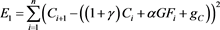
In Figure 1, I have plotted a fit of T to three Gompertz functions

$C\left(t\right)=\exp \left(0.5\left(1-\exp \left(-0.5t\right)\right)\right)$ (18)

Figure 1. A fit to Gompertz functions. The upper curve is $C\left(t\right)$ , the middle $GI\left(t\right)$ and the lower curve is $GF\left(t\right)$ . The solid curves are the Gompertz functions and the dots the model T.

$GF\left(t\right)=\exp \left(0.3\left(1-\exp \left(-0.3t\right)\right)\right)$ (19)

$GI\left(t\right)=\exp \left(0.4\left(1-\exp \left(-0.4t\right)\right)\right)$ (20)

From a paper from 1964 [2] we know that solid tumors grow like Gompertz functions. That is the cancer burden is approximately a Gompertz function. Define the error functions

$E_1={\displaystyle \underset{i=1}{\overset{n}{\sum }}}{\left(C_{i+1}-\left(\left(1+\gamma \right)C_i+\alpha G{F}_i+\beta G{I}_i+g_C\right)\right)}^2$ (21)

$E_2={\displaystyle \underset{i=1}{\overset{n}{\sum }}}{\left(G{F}_{i+1}-\left(\delta C_i+\left(1+{\mu }_F\right)G{F}_i+g_F\right)\right)}^2$ (22)

$E_3={\displaystyle \underset{i=1}{\overset{n}{\sum }}}{\left(G{I}_{i+1}-\left(\sigma C_i+\left(1+{\mu }_I\right)G{I}_i+g_I\right)\right)}^2$ (23)

where $C_i,G{F}_i,G{I}_i,i=1,\cdots ,n+1$ are measurements of $C\mathrm{,}GF\mathrm{,}GI$ at equidistant time points $t_i=ϵi,i=1,\cdots ,n+1,ϵ>0$ . We set $C_i=C\left(t_i\right)$ , $G{F}_i=GF\left(t_i\right)$ , $G{I}_i=GI\left(t_i\right)$ Then solve the equations

$\frac{\partial E_1}{\partial \gamma }=0$ (24)

$\frac{\partial E_1}{\partial \alpha }=0$ (25)

$\frac{\partial E_1}{\partial \beta }=0$ (26)

$\frac{\partial E_1}{\partial g_C}=0$ (27)

in unknowns $\gamma \mathrm{,}\alpha \mathrm{,}\beta \mathrm{,}{g}_C$ and

$\frac{\partial E_2}{\partial \delta }=0$ (28)

$\frac{\partial E_2}{\partial {\mu }_F}=0$ (29)

$\frac{\partial E_2}{\partial g_F}=0$ (30)

in unknowns $\delta \mathrm{,}{\mu }_F\mathrm{,}{g}_F$ and

$\frac{\partial E_3}{\partial \sigma }=0$ (31)

$\frac{\partial E_3}{\partial {\mu }_I}=0$ (32)

$\frac{\partial E_3}{\partial g_I}=0$ (33)

in unknowns $\sigma \mathrm{,}{\mu }_I\mathrm{,}{g}_I$ . For instance

$\frac{\partial E_1}{\partial \gamma }=0$ (34)

gives

$\left(1+\gamma \right){\displaystyle \underset{i=1}{\overset{n}{\sum }}}{C}_i^2+\alpha {\displaystyle \underset{i=1}{\overset{n}{\sum }}}{C}_i\cdot G{F}_i+{\displaystyle \underset{i=1}{\overset{n}{\sum }}}{C}_i\cdot G{I}_i+g_C{\displaystyle \underset{i=1}{\overset{n}{\sum }}}{C}_i={\displaystyle \underset{i=1}{\overset{n}{\sum }}}{C}_{i+1}{C}_i$ (35)

The result is

$\gamma =-0.1344$ (36)

$\alpha =0.1656$ (37)

$\beta =-0.4023$ (38)

$g_C=0.598$ (39)

$\delta =0.017$ (40)

$\sigma =0.06485$ (41)

${\mu }_F=-0.2664$ (42)

${\mu }_I=-0.3815$ (43)

$g_F=0.3312$ (44)

$g_I=0.4622$ (45)

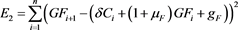
I have also fitted S to two Gompertz functions

$C\left(t\right)=\exp \left(0.5\left(1-\exp \left(-0.5t\right)\right)\right)$ (46)

$GF\left(t\right)=\exp \left(0.3\left(1-\exp \left(-0.3t\right)\right)\right)$ (47)

See Figure 2 and Figure 3. Define error functions

(48)

(49)

Figure 2. A fit of S to a Gompertz functions. The solid curve is the Gompertz function and the dots are the model S.

Figure 3. A fit of S to a Gompertz functions. The solid curve is the Gompertz function and the dots are the model S.

and measurements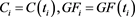. Solve

(50)

(51)

(52)

in unknowns and

(53)

(54)

(55)

in unknowns. The result is

(56)

(57)

(58)

(59)

(60)

(61)

In Maple, there is a command QPSolve that minimizes a quadratic error function with constraints on the signs of the parameters estimated. There are several important monographs relevant to the present paper, see [3] - [8] . There are several publications by the author impacting on the present paper, see [9] - [15] .

2. The Routh Hurwitz Criterion for Maps

We shall derive a well known criterion for stability of a fixed point of a map. To this end define the Möbius transformation

(62)

which maps the left hand plane to the interior of the unit disc. This is because

(63)

implies

(64)

, and

(65)

implies

(66)

Define

(67)

Then

(68)

when lies in the interior of. Also

(69)

(70)

This shows, that g is a bijective map with inverse. Let

(71)

denote the characteristic polynomial of the two by two matrix A in (7). Note, that if and and then and. Here

(72)

(73)

Define

(74)

So if then we have the polynomial

(75)

If this polynomial is a Routh Hurwitz polynomial, i. e. the roots lie in, then the roots of

(76)

lie in the interior of the unit circle. Now compute

(77)

and

(78)

Also

(79)

If

(80)

and the fixed point of S is stable, then by the Routh Hurwitz criterion

(81)

(82)

But this implies, by adding these two inequalities, that

(83)

However, then

(84)

A contradiction to (80). So if is stable, then. Assume now that. If is stable, then

(85)

by the Routh Hurwitz criterion. We shall find the fixed points of S, with. From the second coordinate find

(86)

Then the first coordinate gives

(87)

But the denominator is positive if is stable, by the above. Hence the treatment benefits the patient, because we assume that, and

(88)

and we are lowering by.

Now suppose

(89)

The assumption implies that -1 is a root of

Since, we have

(90)

We claim that is stable, when. But then and are the distinct eigenvalues of A. So there is a change of basis matrix D such that

(91)

Clearly both

(92)

and

(93)

have unique fixed points and and we clearly have

(94)

We need the following definition.

Definition. A fixed point of is stable if given an open neighbourhood of there exists an open neighbourhood of such that for all

(95)

for all. A fixed point is unstable if it is not stable.

Now observe, that

(96)

(97)

Notice that

(98)

in the max norm

(99)

because

(100)

But now stability follows from the estimate

(101)

and this implies that is stable, because S and are conjugate:

(102)

If, then we get the estimate when

(103)

as. So is unstable and since and S are conjugate, is unstable.

3. Models of Cancer Growth

Consider the mapping

(104)

where

(105)

and

(106)

The matrix here is denoted A. T maps to itself. g is a vector of birth rates and. The. Finally . Also put

(107)

(108)

(109)

(110)

(111)

(112)

C is cancer are growth factors and are growth inhibitors,.

Proposition 1 The characteristic polynomial of A is

(113)

(114)

Proof. With,

(115)

(116)

Decompose after the last column to obtain, assuming the formula for holds

(117)

(118)

(119)

(120)

(121)

(122)

(123)

Suppose henceforth, that

(124)

Then the characteristic polynomial of A is

(125)

So the eigenvalues are and since

(126)

is a factor of, then

(127)

are eigenvalues of A, where

(128)

(129)

For the moment assume. Define the matrix of eigenvectors of A by

(130)

We shall find formulas for the complements

(131)

of D and the determinant of D,.

Proposition 2 For we have

(132)

For

(133)

Proof. Suppose. We are deleting row r. So in column there is only one nonzero element. Decomposing after this column and then after row one we get a matrix with zeroes under the diagonal. The signs here are

(134)

is the sign on the complement and is the sign on the complement to. It is in row and column and we delete two rows. is the sign on. Hence

(135)

which is what we wanted to prove.

Now suppose that. For we get a matrix with zeroes under the diagonal, so

(136)

Now consider the case. Write. After decomposing after rows and row one column two in we are left with

(137)

Decompose after rows, to get

(138)

which gives

(139)

The proposition follows, because

(140)

Proposition 3

(141)

Proof. We have

(142)

Initially let. Now

(143)

when and

(144)

when. Now decompose after the last column to get

(145)

If

(146)

(in the statement of the proposition) we get

(147)

Now we shall use induction over q to prove the formula in the statement of the proposition. Decompose after the last row

(148)

(149)

(150)

(151)

In B we have decomposed after and then after the rows and in the remaining matrix decomposed after row p and column. The signs here are

(152)

The proposition follows.

The aim of our computations is to show that there exists an affine vector field X on such that the time one map is

(153)

Let denote an integral curve of X through. Then we shall find a formula for

(154)

First notice that

(155)

if

(156)

and

(157)

which we assume. We have used that

(158)

So the eigenvectors in D are linearly independent, hence

(159)

Now define when

(160)

where. The flow of Y is

(161)

(162)

where we denote the last vector. This is readily shown by differentiating with respect to t

(163)

(164)

(165)

Now we get

(166)

(167)

(168)

It follows that is the flow of Y. Now require

(169)

that is

(170)

We shall require

(171)

because then the time one map of Y is

(172)

Now define

(173)

Then the flows of X and Y are related by

(174)

But then the time one map of X is

(175)

which is what we wanted.

Theorem 4 Assume, that

(176)

and

(177)

We have the formula

(178)

(179)

(180)

(181)

Proof. We use the formula

(182)

(183)

(184)

We have

(185)

and then

(186)

for and for

(187)

We shall write

(188)

and then we have

(189)

When then

(190)

while for we have

(191)

Notice that

(192)

Continuing from (184)

(193)

(194)

(195)

(196)

(197)

So this gives the first term in

(198)

Note that

(199)

Now we have

(200)

(201)

(202)

Hence the contribution is from (184)

(203)

(204)

and the contribution is

(205)

So

(206)

(207)

(208)

(209)

The theorem follows.

Now suppose that. Then

(210)

. We shall require that. Now define the matrix

(211)

The first column is denoted, the second is denoted. Here, both in. Notice that

(212)

(213)

(214)

(215)

Now as in [1] we get

(216)

(217)

(218)

(219)

and similarly

(220)

(221)

(222)

So

(223)

because we assume that. Exactly as before we get

Proposition 5 For

(224)

and for

(225)

Also

(226)

Finally

(227)

since

(228)

Proof. The proposition follows immediately from proposition 2 and 3.

The flow of

(229)

is, for

(230)

We want to have that this equals for, the matrix

(231)

Thus

(232)

(233)

Remember the formula

(234)

Define when.

(235)

where. The flow of Y is

(236)

(237)

where the last vector is denoted. To see this compute

(238)

(239)

Now we also get

(240)

(241)

So is the flow of Y. We need to have

(242)

because then the time one map of Y is

(243)

Then define

(244)

The flows are related by

(245)

But then the time one map of X is

(246)

which is what we intended to find.

Theorem 6 When then

(247)

(248)

(249)

Proof. We have the following computation

(250)

(251)

And we want to have

(252)

(253)

that is

(254)

But we have arranged that

(255)

so we get

(256)

(257)

Denote the two by two matrix in the last line

(258)

We can also compute the first term in

(259)

omitting the factor

(260)

(261)

(262)

(263)

hence the first term in

(264)

Now

(265)

(266)

The contribution is omitting the factor

(267)

(268)

(269)

(270)

The contribution is, omitting the factor

(271)

(272)

(273)

(274)

where

(275)

The theorem follows.

Now assume that. Define

(276)

Proposition 7 For q odd and

(277)

and for and q odd

(278)

For q even and

(279)

and for and q even

(280)

Also

(281)

when q is odd and

(282)

when q is even.

Proof. (277) q odd. We are deleting the row r with. Decompose after that column with in it and row one column two. The sign on is

(283)

The first sign here is the sign when decomposing after row, except the row with. The second sign is the sign on the complement to. The third sign is the sign on. The last sign is the sign on in column r and row one. (277) follows. Now let. Write. Decomposing after rows to give

(284)

We have the sign

(285)

on. And we have the sign

(286)

on column and row one. Hence the formula. is obvious. And the formulas for q even follow similarly. (281) q odd. First let and. Then

(287)

For we get

(288)

We have, decomposing after the last column

(289)

(290)

(291)

(292)

Here

(293)

For q even we get

(294)

Now decompose after the last column

(295)

Now we get decomposing after the last column

(296)

(297)

(298)

(299)

where

(300)

In the determinant B, we have decomposed after row 2 to. In the remaining determinant decompose after row one and column. The proposition follows.

Define for and

(301)

From Proposition 7, we get

Proposition 8 For q odd and

(302)

and for q odd and

(303)

For q even and

(304)

and for q even and

(305)

Also for q odd and

(306)

and for q odd and

(307)

For q even and

(308)

and for q even and

(309)

Finally for q odd

(310)

and

(311)

for q even.

4. An ODE Model

In [1] we also considered a three dimensional ODE model of cancer growth in the variables cancer, growth factors and growth inhibitors, respectively. Analogous to what we did in section three define a mass action kinetic system

(312)

(313)

(314)

(315)

(316)

(317)

Here the complexes are, , , , , This defines the rate constants. For a reaction

(318)

the forward reaction rate is denoted and the reverse reaction rate is denoted. The differential equations are

(319)

(320)

(321)

We shall find a polynomial giving candidates of singular points of this vector field.

From, we find

(322)

where. From, we find

(323)

for. Inserted into we get

(324)

We can then multiply with

(325)

and define the constants

(326)

to obtain the polynomial of degree

(327)

(328)

if we assume that. There is a relation between the ODE model of this chapter, with vector field

(329)

and the discrete dynamical system of section three, see also [1] . Linearize the vector field at a singular point and set

(330)

Also define the Euler map

(331)

for. This is an approximation to the flow of h. If we let

(332)

(333)

(334)

(335)

(336)

(337)

and

(338)

(339)

then you obtain a discrete model T of section three.

Example Let and define the rate constants and,. Then there are two positive singular points.

5. Summary

In this paper, we considered a discrete mathematical model and an ODE model of cancer growth in the variables cancer, growth factors and growth inhibitors, respectively. We have shown that this model is a threshold model. If and

(340)

then cancer grows, and if the reverse inequality holds, cancer is eliminated. We also proposed personalized treatment using the simple model of cancer growth in the introduction and the ODE model of section four.

Conflicts of Interest

The authors declare no conflicts of interest.

References

[1]	Larsen, J.C. (2017) Models of Cancer Growth. Journal of Applied Mathematics and Computing, 53, 615-643.
[2]	Laird, A.K. (1964) Dynamics of Cancer Growth. British Journal of Cancer, 18, 490-502. https://doi.org/10.1038/bjc.1964.55
[3]	Adam, J.A. and Bellomo, N. (1997) A Survey of Models for Tumor-Induced Immune System Dynamics. Birkh?user, Boston.
[4]	Geha, R. and Notarangelo, L. (2012) Case Studies in Immunology. Garland Science, New York, London.
[5]	Marks, F., Klingmüller, U. and Müller-Decker, K. (2009) Cellular Signal Processing. Garland Science, Heidelberg.
[6]	Molina-Paris, C. and Lythe, G. (2011) Mathematical Models and Immune Cell Biology. Springer Verlag, Beilin. https://doi.org/10.1007/978-1-4419-7725-0
[7]	Murphy, K. (2012) Immuno Biology. 8th Edition, Garland Science, New York, London.
[8]	Rees, R.C. (2014) Tumor Immunology and Immunotherapy. Oxford University Press, Oxford.
[9]	Larsen, J.C. (2016) Hopf Bifurcations in Cancer Models. JP Journal of Applied Mathematics, 14, 1-31.
[10]	Larsen, J.C. (2017) A Mathematical Model of Adoptive T Cell Therapy. JP Journal of Applied Mathematics, 15, 1-33.
[11]	Larsen, J.C. (2016) Fundamental Concepts in Dynamics. Survey Article.
[12]	Larsen, J.C. (2017) The Bistability Theorem in a Cancer Model. International Journal of Biomathematics. (To appear)
[13]	Larsen, J.C. (2016) The Bistability Theorem in a Model of Metastatic Cancer. Applied Mathematics, 7, 1183-1206. https://doi.org/10.4236/am.2016.710105
[14]	Larsen, J.C. (2017) A Study on Multipeutics. Applied Mathematics, 8, 746-773. https://doi.org/10.4236/am.2017.85059
[15]	Larsen, J.C. (2017) A Mathematical Model of Immunity. JP Journal of Applied Mathematics. (To appear)