Asymptotic Stability of a Series-Parallel Repairable System Consisting of Three-Unit with Multiple Vacations of a Repairman

Tursunjan Keyim, Abdukerim Haji

College of Mathematics and System Sciences, Xinjiang University, Urumqi, China.

DOI: 10.4236/jamp.2017.51018                

Abstract

We study a series-parallel repairable system consisting of three units with multiple vacations of a repairman. We first show that all points on the imaginary axis except zero belong to the resolvent set of the operator and zero is an eigenvalue of the operator, and then we prove that the semigroup generated by the operator is irreducible. By combining these results with our previous result we deduce that the dynamic solution of the system converges strongly to its steady-state solution. Thus we obtain asymptotic stability of the dynamic solution of the system.

Keywords

Series-Parallel Repairable System, C₀-Semigroup, Irreducibility, Asymptotic Stability

1. Introduction

The series-parallel repairable system consisting of three units, as one of the important systems in reliability applications, has been studied in previous literatures. Li et al. [1] studied a repairable system with three units and two different repair facilities, and obtained the explicit expressions of the state probabilities of the system and the steady-state reliability of the system. Kovalenko [2] investigated a three-component system consisting of one master control element and two slave elements with priority serving by a single repair facility, and obtained the failure frequency and the average up-time. In those literatures, the authors assumed that the failed unit would be immediately repaired and as good as new after repair. But in practice, due to various reasons, the failed unit cannot be immediately repaired. In addition, in the case of good units, the repairman leaves for a vacation or does other work, which can increase the profit of the system. From this point, to study reliability of repairable systems with a repairman who can take a vacation or can do other work is important in terms of theory and practice. Hu et al. [3] considered a series-parallel repairable system with three units and multiple vacations of a repairman; they obtained the reliability indices of the system by using the method of supplement variables, the vector Markov progress method and the tool of the Laplace transform. They used the dynamic solution in calculating the availability and the reliability. But they did not discuss the existence of the dynamic solution and the asymptotic stability of the dynamic solution. Haji et al. [4] proved that the above system has a unique nonnegative dynamic solution under the assumption 1.1 by using results from the theory of positive operators and semigroups that can be found in [5] and [6] . In this paper, we further study this system and prove that the dynamic solution converges strongly to the steady state solution under the assumption 1.1.

2. Fundamental Principles

Our main focus in this paper is on the asymptotic stability of the dynamic solution of the system. We prove that the dynamic solution converges strongly to the steady state solution which is the eigenfunction corresponding to eigenvalue 0 of the system operator. To this purpose we first prove that 0 is an eigenvalue of the system operator we obtain that all points on the imaginary axis except zero belong to the resolvent set of the system operator, and then we prove that the semigroup generated by the operator is irreducible. By combining these results with our previous result we deduce that the dynamic solution of the system converges strongly to its steady-state solution.

According to [3] , the series-parallel repairable system consisting of three-unit with multiple vacations of a repair-man can be described by the following system of partial differential equations with integral boundary conditions:

$\left(\frac{\partial }{\partial t}+\frac{\partial }{\partial x}\right)p_0\left(t,x\right)=-\left[\lambda +2\mu +\alpha \left(x\right)\right]p_0\left(t,x\right),$ (1)

$\left(\frac{\partial }{\partial t}+\frac{\partial }{\partial x}\right)p_1\left(t,x\right)=-\left[\lambda +\mu +\alpha \left(x\right)\right]p_1\left(t,x\right)+2\mu p_0\left(t,x\right),$ (2)

$\left(\frac{\partial }{\partial t}+\frac{\partial }{\partial x}\right)p_2\left(t,x\right)=-\alpha \left(x\right)p_2\left(t,x\right)+\lambda p_0\left(t,x\right),$ (3)

$\left(\frac{\partial }{\partial t}+\frac{\partial }{\partial x}\right)p_3\left(t,x\right)=-\alpha \left(x\right)p_3\left(t,x\right)+\lambda p_1\left(t,x\right),$ (4)

$\left(\frac{\partial }{\partial t}+\frac{\partial }{\partial x}\right)p_4\left(t,x\right)=-\alpha \left(x\right)p_4\left(t,x\right)+\mu p_1\left(t,x\right),$ (5)

$\left(\frac{\partial }{\partial t}+\frac{\partial }{\partial y}\right)p_5\left(t,y\right)=-\left[\lambda +\mu +b_2\left(y\right)\right]p_5\left(t,y\right),$ (6)

$\left(\frac{\partial }{\partial t}+\frac{\partial }{\partial y}\right)p_6\left(t,y\right)=-b_1\left(y\right)p_6\left(t,y\right),$ (7)

$\left(\frac{\partial }{\partial t}+\frac{\partial }{\partial y}\right)p_7\left(t,y\right)=-b_1\left(y\right)p_7\left(t,y\right),$ (8)

$\left(\frac{\partial }{\partial t}+\frac{\partial }{\partial y}\right)p_8\left(t,y\right)=-b_2\left(y\right)p_8\left(t,y\right)+\mu p_5\left(t,y\right),$ (9)

$\left(\frac{\partial }{\partial t}+\frac{\partial }{\partial y}\right)p_9\left(t,y\right)=-b_2\left(y\right)p_9\left(t,y\right)+\lambda p_5\left(t,y\right),$ (10)

with the boundary conditions

$\begin{array}{l}{p}_0\left(t,0\right)={\displaystyle {\int }_0^{+\infty }\alpha \left(x\right)p_0\left(t,x\right)}\text{d}x+{\displaystyle {\int }_0^{+\infty }{b}_2\left(y\right)p_5\left(t,y\right)}\text{d}y\\ +{\displaystyle {\int }_0^{+\infty }{b}_1\left(y\right)p_6\left(t,y\right)}\text{d}y+\delta \left(t\right),\end{array}$ (11)

$p_1\left(t,0\right)=p_2\left(t,0\right)=p_3\left(t,0\right)=p_4\left(t,0\right)=0,$ (12)

$\begin{array}{l}{p}_5\left(t,0\right)={\displaystyle {\int }_0^{+\infty }\alpha \left(x\right)p_1\left(t,x\right)}\text{d}x+{\displaystyle {\int }_0^{+\infty }{b}_1\left(y\right)p_7\left(t,y\right)}\text{d}y\\ +{\displaystyle {\int }_0^{+\infty }{b}_2\left(y\right)p_8\left(t,y\right)}\text{d}y,\end{array}$ (13)

$p_6\left(t,0\right)={\displaystyle {\int }_0^{+\infty }\alpha \left(x\right)p_2\left(t,x\right)}\text{d}x+{\displaystyle {\int }_0^{+\infty }{b}_2\left(y\right)p_9\left(t,y\right)}\text{d}y,$ (14)

$p_7\left(t,0\right)={\displaystyle {\int }_0^{+\infty }\alpha \left(x\right)p_3\left(t,x\right)}\text{d}x,$ (15)

$p_8\left(t,0\right)={\displaystyle {\int }_0^{+\infty }\alpha \left(x\right)p_4\left(t,x\right)}\text{d}x,$ (16)

$p_9\left(t,0\right)=0,$ (17)

and the initial conditions

$p_0\left(0,x\right)=\delta \left(x\right),$ (18)

$p_i\left(0,x\right)=0,i=1,2,3,4,$ (19)

$p_i\left(0,y\right)=0,i=5,6,7,8,9,$ (20)

$\delta \left(x\right)=\{\begin{array}{c}1,x=0,\\ 0,x\ne 0,\end{array}$ (21)

where $\left(t,x\right)\in \left[0,+\infty \right)\times \left[0,+\infty \right),\left(t,y\right)\in \left[0,+\infty \right)\times \left[0,+\infty \right)$ ; and the symbols in the equations have the following meaning.

$p_0\left(t,x\right)\text{d}x:$ the probability that at time t all the three units are operating, the repairman is in vacation, the system is good and the elapsed vacation time lies in $\left[x,x+\text{d}x\right)$ ;

$p_1\left(t,x\right)\text{d}x:$ the probability that at time $t$ unit 1 and one of unit 2 and unit 3 are operating, another one is waiting for repair, the repairman is in vacation, the system is good and the elapsed vacation time lies in $\left[x,x+\text{d}x\right)$ ;

$p_2\left(t,x\right)\text{d}x:$ the probability that at time $t$ unit 2 and unit 3 are temporarily halted, unit 1 is waiting for repair, the repairman is in vacation, the system is down and the elapsed repair time lies in $\left[x,x+\text{d}x\right)$ ;

$p_3\left(t,x\right)\text{d}x:$ the probability that at time $t$ one of unit 2 and unit 3 is temporarily halted, another one is waiting for repair, unit 1 is also waiting for repair , the repairman is in vacation, the system is down and the elapsed vacation time lies in $\left[x,x+\text{d}x\right)$ ;

$p_4\left(t,x\right)\text{d}x:$ the probability that at time $t$ unit 1 is temporarily halted, unit 2 and unit 3 are waiting for repair, is also waiting for repair, the repairman is in vacation, the system is down and the elapsed vacation time lies in $\left[x,x+\text{d}x\right)$ ;

$p_5\left(t,y\right)\text{d}y:$ the probability that at time $t$ unit 1 and one of unit 2 and unit 3 are operating, another one being repaired by the repairman, the system is good and the elapsed repair time of unit 2 or unit 3 lies in $\left[y,y+\text{d}y\right)$ ;

$p_6\left(t,y\right)\text{d}y:$ the probability that at time $t$ unit 2 and unit 3 are temporarily halted, unit 1 being repaired, the system is down and the elapsed repair time of unit 1 lies in $\left[y,y+\text{d}y\right)$ ;

$p_7\left(t,y\right)\text{d}y:$ the probability that at time $t$ one of unit 2 and unit 3 are temporarily halted, another one is waiting for repair, unit 1 being repaired, the system is down and the elapsed repair time of unit 1 lies in $\left[y,y+\text{d}y\right)$ ;

$p_8\left(t,y\right)\text{d}y:$ the probability that at time $t$ unit 1 is temporarily halted, one of unit 2 and unit 3 is waiting for repair, another one being repaired by the repairman, the system is down and the elapsed repair time of unit 2 or unit 3 lies in $\left[y,y+\text{d}y\right)$ ;

$p_9\left(t,y\right)\text{d}y:$ the probability that at time $t$ unit 1 is waiting for repair, one of unit 2 and unit 3 is temporarily halted, another one being repaired by the repairman, the system is down and the elapsed repair time of unit 2 or unit 3 lies in $\left[y,y+\text{d}y\right)$ ;

$\lambda ,\mu :$ positive constants; $\alpha \left(x\right):$ the vacation rate function;

$b_1\left(y\right),b_2\left(y\right):$ the repair rate function of unit 1 and unit 2 (or unit 3).

Assumption 1.1: The functions $\alpha \left(x\right)$ and $b_i\left(y\right):\left[0,+\infty \right)\to \left[0,+\infty \right)\left(i=1,2\right)$ are measurable and bounded such that

$\alpha ={\lim }_{x\to +\infty }\alpha \left(x\right),b_i={\lim }_{y\to +\infty }{b}_i\left(y\right),b_{\infty }=\min \left(\alpha ,b_1,b_2\right).$ (22)

In [4] , the authors transformed the system into an abstract Cauchy problem [5] , Def. II.6.1] on the Banach space $\left(X,\Vert .\Vert \right)$

$\{\begin{array}{l}\frac{\text{d}p\left(t\right)}{\text{d}t}=Ap\left(t\right),t\in \left[0,\infty \right),\hfill \\ p\left(0\right)={\left(\delta \left(x\right),0,0,0,0,0,0,0,0,0\right)}^{\text{T}}\in X,\hfill \end{array}$ (23)

where $X={\left(L_x^1\left(\left[0,+\infty \right)\right)\right)}^5\times {\left(L_y^1\left(\left[0,+\infty \right)\right)\right)}^5$ with norm

$\Vert p\Vert ={\displaystyle {\sum }_{i=0}^4{\Vert p_i\Vert }_{L_x^1\left(\left[0,+\infty \right)\right)}}+{\displaystyle {\sum }_{i=5}^9{\Vert p_i\Vert }_{L_y^1\left(\left[0,+\infty \right)\right)}},$ (24)

$p={\left(p_0\left(x\right),p_1\left(x\right),p_2\left(x\right),p_3\left(y\right),p_4\left(x\right),p_5\left(y\right),p_6\left(y\right),p_7\left(y\right),p_8\left(y\right),p_9\left(y\right)\right)}^t\in X,$ (25)

$Ap=A_{m}p,D\left(A\right)=\left\{p\in D\left(A_m\right)|Ep=Fp\right\}$ (26)

$A_m=\left(\begin{array}{llllllllll}{A}_{1,1}\hfill & 0\hfill & 0\hfill & 0\hfill & 0\hfill & 0\hfill & 0\hfill & 0\hfill & 0\hfill & 0\hfill \\ 2\mu \hfill & A_{2,2}\hfill & 0\hfill & 0\hfill & 0\hfill & 0\hfill & 0\hfill & 0\hfill & 0\hfill & 0\hfill \\ \lambda \hfill & 0\hfill & A_{3,3}\hfill & 0\hfill & 0\hfill & 0\hfill & 0\hfill & 0\hfill & 0\hfill & 0\hfill \\ 0\hfill & \lambda \hfill & 0\hfill & A_{4,4}\hfill & 0\hfill & 0\hfill & 0\hfill & 0\hfill & 0\hfill & 0\hfill \\ 0\hfill & \mu \hfill & 0\hfill & 0\hfill & A_{5,5}\hfill & 0\hfill & 0\hfill & 0\hfill & 0\hfill & 0\hfill \\ 0\hfill & 0\hfill & 0\hfill & 0\hfill & 0\hfill & A_{6,6}\hfill & 0\hfill & 0\hfill & 0\hfill & 0\hfill \\ 0\hfill & 0\hfill & 0\hfill & 0\hfill & 0\hfill & 0\hfill & A_{7,7}\hfill & 0\hfill & 0\hfill & 0\hfill \\ 0\hfill & 0\hfill & 0\hfill & 0\hfill & 0\hfill & 0\hfill & 0\hfill & A_{8,8}\hfill & 0\hfill & 0\hfill \\ 0\hfill & 0\hfill & 0\hfill & 0\hfill & 0\hfill & \mu \hfill & 0\hfill & 0\hfill & A_{9,9}\hfill & 0\hfill \\ 0\hfill & 0\hfill & 0\hfill & 0\hfill & 0\hfill & \lambda \hfill & 0\hfill & 0\hfill & 0\hfill & A_{10,10}\hfill \end{array}\right),$ (27)

$D\left(A_m\right)={\left(W_x^{1,1}\left[0,\infty \right]\right)}^5\times {\left(W_y^{1,1}\left[0,\infty \right]\right)}^5$ (28)

$\begin{array}{l}{A}_{1,1}=-\frac{\text{d}}{\text{d}x}-\left[\lambda +2\mu +\alpha \left(x\right)\right],\\ A_{22}=-\frac{\text{d}}{\text{d}x}-\left[\lambda +\mu +\alpha \left(x\right)\right],\\ A_{33}=A_{44}=A_{55}=-\frac{\text{d}}{\text{d}x}-\alpha \left(x\right),\end{array}$ (29)

$\begin{array}{l}{A}_{6,6}=-\frac{\text{d}}{\text{d}y}-\left[\lambda +\mu +b_2\left(y\right)\right],\\ A_{7,7}=A_{8,8}=-\frac{\text{d}}{\text{d}y}-b_1\left(y\right),\\ A_{9,9}=A_{10,10}=-\frac{\text{d}}{\text{d}y}-b_2\left(y\right),\end{array}$ (30)

(31)

$\begin{array}{l}{\phi }_1:L_x^1\left[0,\infty \right)\to C,f\to {\phi }_1\left(f\right)={\displaystyle {\int }_0^{\infty }\alpha \left(x\right)f\left(x\right)}\text{d}x,\\ {\phi }_i:L_y^1\left[0,\infty \right)\to C,f\to {\phi }_i\left(f\right)={\displaystyle {\int }_0^{\infty }{b}_i\left(y\right)f\left(y\right)}\text{d}y\left(i=1,2\right).\end{array}$ (32)

3. The Main Result

To prove our main result on the asymptotic stability of the dynamic solution of system, we first prove the some lemmas.

In [7] , A. Haji and A. Radl gave the following result.

Lemma 2.1: Let $\gamma \in \rho \left(A_0\right)$ , then

(i) $\gamma \in {\sigma }_p\left(A\right)\iff 1\in {\sigma }_p\left(F{D}_{\gamma }\right)$ .

(ii) If $\gamma \in \rho \left(A_0\right)$ and there exists ${\gamma }_0\in ℂ$ such that $1\in \sigma \left(F{D}_{{\gamma }_0}\right)$ , then

$\gamma \in \sigma \left(A\right)\iff 1\in \sigma \left(F{D}_{\gamma }\right)$ .

In our situation the operator $F{D}_{\gamma }$ is 10 ´ 10-matrix, see [4] .

Lemma 2.2: For the operator $\left(A,D\left(A\right)\right)$ we have $0\in {\sigma }_p\left(A\right)$ .

Proof: All the entries of $F{D}_0$ are positive and one can compute each column sum of the 10 ´ 10-matrix $F{D}_0$ as follows:

$\begin{array}{l}{a}_{11}\left(0\right)+a_{61}\left(0\right)+a_{71}\left(0\right)+a_{81}\left(0\right)+a_{91}\left(0\right)\\ ={\displaystyle {\int }_0^{+\infty }c\left(x\right)e^{-\left(\lambda +2\mu \right)x-{\displaystyle {\int }_0^{x}c\left(\tau \right)}\text{d}\tau }}\text{d}x+2{\displaystyle {\int }_0^{+\infty }c\left(x\right)e^{-\left(\lambda +\mu \right)x-{\displaystyle {\int }_0^{x}c\left(\tau \right)}\text{d}\tau }\left(1-e^{-\mu x}\right)}\text{d}x\\ +\frac{\lambda }{\lambda +2\mu }{\displaystyle {\int }_0^{+\infty }c\left(x\right)e^{-{\displaystyle {\int }_0^{x}c\left(\tau \right)}\text{d}\tau }\left(1-e^{-\left(\lambda +2\mu \right)x}\right)}\text{d}x\\ +2\lambda {\displaystyle {\int }_0^{+\infty }c\left(x\right)e^{-{\displaystyle {\int }_0^{x}c\left(\tau \right)\text{d}\tau }}\left[\frac{1}{\lambda +\mu }\left(1-e^{-\left(\lambda +2\mu \right)x}\right)-\frac{1}{\lambda +2\mu }\left(1-e^{-\left(\lambda +2\mu \right)}\right)\right]}\text{d}x\\ +2\mu {\displaystyle {\int }_0^{+\infty }c\left(x\right)e^{-{\displaystyle {\int }_0^{x}c\left(\tau \right)\text{d}\tau }}\left[\frac{1}{\lambda +\mu }\left(1-e^{-\left(\lambda +2\mu \right)x}\right)-\frac{1}{\lambda +2\mu }\left(1-e^{-\left(\lambda +2\mu \right)x}\right)\right]}\text{d}x\\ =\left(2-\frac{\lambda }{\lambda +2\mu }-\frac{2\mu }{\lambda +\mu }\right){\displaystyle {\int }_0^{+\infty }c\left(x\right)e^{-\left(\lambda +\mu \right)-{\displaystyle {\int }_0^{x}c\left(\tau \right)\text{d}\tau }}}\text{d}x\\ +\left(-1-\frac{\lambda }{\lambda +2\mu }+\frac{2\lambda }{\lambda +2\mu }+\frac{2\mu }{\lambda +2\mu }\right){\displaystyle {\int }_0^{+\infty }c\left(x\right)e^{-\left(\lambda +2\mu \right)-{\displaystyle {\int }_0^{x}c\left(\tau \right)\text{d}\tau }}\text{d}x}\\ +\left(\frac{\lambda }{\lambda +2\mu }+\frac{2\lambda }{\lambda +\mu }-\frac{2\lambda }{\lambda +2\mu }+\frac{2\mu }{\lambda +2\mu }-\frac{2\mu }{\lambda +2\mu }\right)=1,\end{array}$ (33)

$a_{7,3}\left(0\right)={\displaystyle {\int }_0^{+\infty }\alpha \left(x\right)e^{-{\displaystyle {\int }_0^x\alpha \left(\tau \right)}\text{d}\tau }}\text{d}x=1$ (34)

$a_{8,4}\left(0\right)={\displaystyle {\int }_0^{+\infty }\alpha \left(x\right)e^{-{\displaystyle {\int }_0^x\alpha \left(\tau \right)}\text{d}\tau }}\text{d}x=1$ (35)

$a_{9,5}\left(0\right)={\displaystyle {\int }_0^{+\infty }\alpha \left(x\right)e^{-{\displaystyle {\int }_0^x\alpha \left(\tau \right)}\text{d}\tau }}\text{d}x=1$ (36)

$\begin{array}{l}{a}_{62}\left(0\right)+a_{82}\left(0\right)+a_{92}\left(0\right)\\ ={\displaystyle {\int }_0^{+\infty }c\left(x\right)e^{-\left(\lambda +2\mu \right)x-{\displaystyle {\int }_0^{x}c\left(\tau \right)}\text{d}\tau }}\text{d}x\\ +\frac{\lambda }{\lambda +\mu }{\displaystyle {\int }_0^{+\infty }c\left(x\right)e^{-{\displaystyle {\int }_0^{x}c\left(\tau \right)}\text{d}\tau }\left(1-e^{-\left(\lambda +\mu \right)x}\right)}\text{d}x\\ +\frac{\mu }{\lambda +\mu }{\displaystyle {\int }_0^{+\infty }c\left(x\right)e^{-{\displaystyle {\int }_0^{x}c(\tau )}\text{d}\tau }\left(1-e^{-\left(\lambda +\mu \right)x}\right)}\text{d}x\\ ={\displaystyle {\int }_0^{+\infty }c\left(x\right)e^{-\left(\lambda +\mu \right)x-{\displaystyle {\int }_0^{x}c\left(\tau \right)}\text{d}\tau }}\text{d}x+{\displaystyle {\int }_0^{+\infty }c\left(x\right)e^{-{\displaystyle {\int }_0^{x}c\left(\tau \right)\text{d}\tau }}}\text{d}x\\ -{\displaystyle {\int }_0^{+\infty }c\left(x\right)e^{-\left(\lambda +\mu \right)x-{\displaystyle {\int }_0^{x}c\left(\tau \right)\text{d}\tau }}}\text{d}x=1,\end{array}$ (37)

$\begin{array}{l}{a}_{16}\left(0\right)+a_{66}\left(0\right)+a_{76}\left(0\right)\\ ={\displaystyle {\int }_0^{+\infty }{b}_2\left(y\right)e^{-\left(\lambda +\mu \right)y-{\displaystyle {\int }_0^y{b}_2\left(y\right)}\text{d}\tau }}\text{d}y+\frac{\mu }{\lambda +\mu }{\displaystyle {\int }_0^{+\infty }{b}_2\left(y\right)e^{-{\displaystyle {\int }_0^y{b}_2\left(\tau \right)\text{d}}\tau }\left(1-e^{-\left(\lambda +\mu \right)y}\right)}\text{d}y\\ +\frac{\lambda }{\lambda +\mu }{\displaystyle {\int }_0^{+\infty }{b}_2\left(y\right)e^{-{\displaystyle {\int }_0^y{b}_2\left(\tau \right)}\text{d}\tau }\left(1-e^{-\left(\lambda +\mu \right)y}\right)}\text{d}y=1,\end{array}$ (38)

$a_{1,7}\left(0\right)={\displaystyle {\int }_0^{+\infty }{b}_1\left(y\right)e^{-{\displaystyle {\int }_0^y{b}_1\left(\tau \right)}\text{d}\tau }}\text{d}y=1,$ (39)

$a_{6,8}\left(0\right)={\displaystyle {\int }_0^{+\infty }{b}_1\left(y\right)e^{-{\displaystyle {\int }_0^y{b}_1\left(\tau \right)}\text{d}\tau }}\text{d}y=1,$ (40)

$a_{6,9}\left(0\right)={\displaystyle {\int }_0^{+\infty }{b}_2\left(y\right)e^{-{\displaystyle {\int }_0^y{b}_2\left(\tau \right)}\text{d}\tau }}\text{d}y=1,$ (41)

$a_{7,10}\left(0\right)={\displaystyle {\int }_0^{+\infty }{b}_2\left(y\right)e^{-{\displaystyle {\int }_0^y{b}_2\left(\tau \right)}\text{d}\tau }}\text{d}y=1.$ . (42)

From (33)-(42) we know that the matrix $F{D}_0$ is column stochastic and thus $1\in {\sigma }_p\left(F{D}_0\right)$ . Applying Lemma 2.1(i), we immediately obtain $0\in {\sigma }_p\left(A\right)$ .

Using Lemma 2.1(ii) we can show that 0 is the only spectral value of A on the imaginary axis.

Lemma 2.3: The spectrum $\sigma \left(A\right)$ of a satisfies $\sigma \left(A\right){{\displaystyle \cap }}^{\text{}}iR=\left\{0\right\}$ .

Proof: If $b\in ℝ,b\ne 0$ , then it is not difficult to derive that $\Vert F{D}_{ai}\Vert <1$ , thus the spectral radius fulfills $r\left(F{D}_{ai}\right)\le \Vert F{D}_{ai}\Vert <1$ . This implies $1\in \rho \left(F{D}_{ai}\right)$ . By Lemma 2.1 (ii) we obtain that $ai\notin \sigma \left(A\right)$ for all $a\in R$ , $a\ne 0$ , i.e., $\sigma \left(A\right)\cap iR=\left\{0\right\}$ .

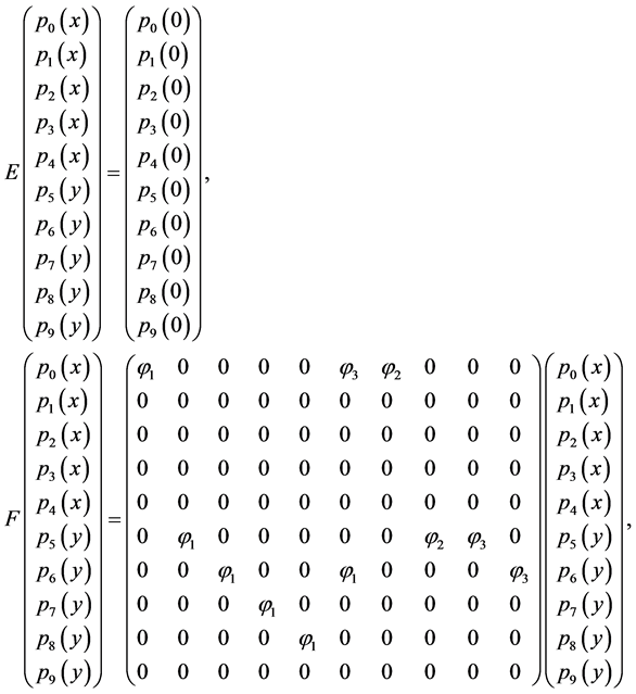
Lemma 2.4: If the operator $\left(A_0,D\left(A_0\right)\right)$ is defined by $A_{0}p=A_{m}p,D\left(A_0\right)=\left\{p\in D\left(A_m\right)|Ep=0\right\},$ then for the set $S=\left\{\gamma \in ℂ|\mathrm{Re}\gamma >-{\mu }_{\infty }\right\}$ we have

$S\subseteq \rho \left(A_0\right)$ (43)

Moreover, if $\gamma \in S$ , then

$R\left(\gamma ,A_0\right)=\left(\begin{array}{cccccccccc}{t}_{1,1}& 0& \oplus & 0& 0& 0& 0& 0& 0& 0\\ t_{2,1}& t_{2,2}& 0& 0& 0& 0& 0& 0& 0& 0\\ t_{3,1}& 0& t_{3,3}& 0& 0& 0& 0& 0& 0& 0\\ t_{4,1}& t_{4,2}& 0& t_{4,4}& 0& 0& 0& 0& 0& 0\\ t_{5,1}& t_{5,2}& 0& 0& t_{5,5}& 0& 0& 0& 0& 0\\ 0& 0& 0& 0& 0& t_{6,6}& 0& 0& 0& 0\\ 0& 0& 0& 0& 0& 0& t_{7,7}& 0& 0& 0\\ 0& 0& 0& 0& 0& 0& 0& t_{8,8}& 0& 0\\ 0& 0& 0& 0& 0& t_{9,6}& 0& 0& t_{9,9}& 0\\ 0& 0& 0& 0& 0& t_{10,6}& 0& 0& 0& t_{10,10}\end{array}\right)$ (44)

where

$t_{1,1}=R\left(\gamma ,D_{11}\right),t_{2,1}=2\mu R\left(\gamma ,D_{22}\right)R\left(\gamma ,D_{11}\right),t_{2,2}=R\left(\gamma ,D_{22}\right),$ (45)

$t_{3,1}=\lambda R\left(\gamma ,D_{33}\right)R\left(\gamma ,D_{11}\right),t_{3,3}=R\left(\gamma ,D_{33}\right),$ (46)

$\begin{array}{l}{t}_{4,1}=2\lambda \mu R\left(\gamma ,D_{44}\right)R\left(\gamma ,D_{22}\right)R\left(\gamma ,D_{11}\right),\\ t_{4,2}=\lambda R\left(\gamma ,D_{44}\right)R\left(\gamma ,D_{22}\right),\\ t_{4,4}=R\left(\gamma ,D_{44}\right),\end{array}$ (47)

$\begin{array}{l}{t}_{5,1}=2{\mu }^{2}R\left(\gamma ,D_{55}\right)R\left(\gamma ,D_{44}\right)R\left(\gamma ,D_{11}\right),\\ t_{5,2}=\mu R\left(\gamma ,D_{55}\right)R\left(\gamma ,D_{22}\right),\\ t_{5,5}=R\left(\gamma ,D_{55}\right),\end{array}$ (48)

$\begin{array}{l}{t}_{6,6}=R\left(\gamma ,D_{66}\right),t_{7,7}=R\left(\gamma ,D_{77}\right),\\ t_{8,8}=R\left(\gamma ,D_{88}\right),t_{9,6}=\mu R\left(\gamma ,D_{99}\right)R\left(\gamma ,D_{66}\right),\end{array}$ (49)

$t_{9,9}=R\left(\gamma ,D_{99}\right),t_{10,6}=\lambda R\left(\gamma ,D_{10,10}\right)R\left(\gamma ,D_{66}\right),t_{10,10}=R\left(\gamma ,D_{10,10}\right).$ (50)

The resolvent operator of the differential operators $D_{i,j,0}$ where $D_{i,j,0}=D_{i,j}$ with domain $D\left(D_{i,j,0}\right)=\left\{g\in W^{1,1}\left(0,+\infty \right):g\left(0\right)=0\right\}$ , $i=1,2,3,4,5,6,7,8,9,10$ , $j=1,2,3,4,5,6,7,8,9,10$ , are given by

$\left(R\left(\gamma ,D_{1,1,0}\right)g\right)\left(x\right)=e^{-\left(\gamma +\lambda +2\mu \right)x-{\displaystyle {\int }_0^x\alpha \left(\tau \right)}\text{d}\tau }{\displaystyle {\int }_0^x{e}^{\left(\gamma +\lambda +2\mu \right)s-{\displaystyle {\int }_0^s\alpha \left(\tau \right)}\text{d}\tau }g\left(s\right)}\text{d}s,$ (51)

$\left(R\left(\gamma ,D_{2,2,0}\right)g\right)\left(x\right)=e^{-\left(\gamma +\lambda +2\mu \right)x-{\displaystyle {\int }_0^x\alpha \left(\tau \right)}\text{d}\tau }{\displaystyle {\int }_0^x{e}^{\left(\gamma +\lambda +\mu \right)s-{\displaystyle {\int }_0^s\alpha \left(\tau \right)}\text{d}\tau }g\left(s\right)}\text{d}s,$ (52)

$\left(R\left(\gamma ,D_{i,i,0}\right)g\right)\left(x\right)=e^{-\gamma x-{\displaystyle {\int }_0^x\alpha \left(\tau \right)}\text{d}\tau }{\displaystyle {\int }_0^x{e}^{\gamma s-{\displaystyle {\int }_0^s\alpha \left(\tau \right)}\text{d}\tau }g\left(s\right)}\text{d}s,i=3,4,5,$ (53)

$\left(R\left(\gamma ,D_{6,6,0}\right)g\right)\left(x\right)=e^{-\left(\gamma +\lambda +\mu \right)x-{\displaystyle {\int }_0^x\alpha \left(\tau \right)}\text{d}\tau }{\displaystyle {\int }_0^x{e}^{\left(\gamma +\lambda +\mu \right)s-{\displaystyle {\int }_0^s\alpha \left(\tau \right)}\text{d}\tau }g\left(s\right)}\text{d}s,$ (54)

$\left(R\left(\gamma ,D_{j,j,0}\right)g\right)\left(y\right)=e^{-\gamma y-{\displaystyle {\int }_0^y{b}_1\left(\tau \right)}\text{d}\tau }{\displaystyle {\int }_0^y{e}^{\gamma s-{\displaystyle {\int }_0^s{b}_1\left(\tau \right)}\text{d}\tau }g\left(s\right)}\text{d}s,j=7,8,$ (55)

$\left(R\left(\gamma ,D_{k,k,0}\right)g\right)\left(y\right)=e^{-\gamma y-{\displaystyle {\int }_0^y{b}_2\left(\tau \right)}\text{d}\tau }{\displaystyle {\int }_0^y{e}^{\gamma s-{\displaystyle {\int }_0^s{b}_2\left(\tau \right)}\text{d}\tau }g\left(s\right)}\text{d}s,k=9,10.$ (56)

Applying the same method as in [7] we can express the resolvent of $A$ in terms of the resolvent of $A_0$ , the Dirichlet operator $D_{\gamma }$ and the boundary operator as follows.

Lemma 2.5: If $\gamma \in \rho \left(A_0\right)\cap \rho \left(A\right)$ , then $R\left(\gamma ,A\right)=R\left(\gamma ,A_0\right)+D_{\gamma }{\left(Id-F{D}_{\gamma }\right)}^{-1}FR\left(\gamma ,A_0\right)$ .

The following property of ${\mathcal{C}}_0$ -semigroup ${\left(T\left(t\right)\right)}_{t\ge 0}$ generated by the system operator $\left(A,D\left(A\right)\right)$ is useful to prove the asymptotic stability of the dynamic solution of the system.

Theorem 2.6: The semigroup ${\left(T\left(t\right)\right)}_{t\ge 0}$ generated by $\left(A,D\left(A\right)\right)$ is irreducible.

Proof: By Lemma 2.4 and Lemma 2.5we can see that $R\left(\gamma ,A\right)$ transforms any positive vector $p\in X$ into a strictly positive vector. Using ( [6] , Def. C-III 3.1) this is equivalent to the irreducibility of the semigroup ${\left(T\left(t\right)\right)}_{t\ge 0}$ generated by $\left(A,D\left(A\right)\right)$ .

Using Lemma 2.2, Lemma 2.3, Theorem 2.6and the same method as in ( [7] , Th. 3.11) we obtain the following result.

Theorem 2.7: The space $X$ can be decomposed into the direct sum

$X=X_1\oplus X_2$ (57)

where $X_1=\text{fix}{\left(T\left(t\right)\right)}_{t\ge 0}=\ker A$ is one-dimensional and spanned by a strictly positive eigenvector $\hat{p}\in \ker A$ of $A$ . In addition, the restriction ${\left(T{\left(t\right)|}_{X_2}\right)}_{t\ge 0}$ is strongly stable.

Corollary 2.8: For all $p\in X$ , there exists $\alpha >0$ , such that

${\lim }_{t\to \infty }T\left(t\right)p=\alpha \hat{p},$ (58)

where $\ker A=\hat{p},\hat{p}\gg 0.$

We now obtain our main result as follows.

Corollary 2.9: The dynamic solution of the system (1)-(20) converges strongly to the steady-state solution as time tends to infinity, that is,

${\lim }_{t\to \infty }p\left(t,.\right)=\alpha \hat{p},$ (59)

where $\alpha >0$ and $\hat{p}$ as in Corollary 2.6.

4. Conclusion

In this paper, we investigated a series-parallel repairable system consisting of three units with multiple vacations of a repairman. The study of the dynamic solution as well as its stability is in demand in terms of theory and practice. We discussed the asymptotic stability of the dynamic solution and showed that the dynamic solution converges strongly to the steady state solution by analyzing the spectral distribution of the system operator and taking into account the irreducibility of the semigroup generated by the system operator.

Acknowledgements

This research was supported by the National Natural Science Foundation of China (No. 11361057).

Conflicts of Interest

The authors declare no conflicts of interest.

References

[1]	Li, W., Alfa, A.S. and Zhao, Y.Q. (l998) Stochastic Analysis of a Repairable System with Three Units and Two Repair Facilities. Microelectronics and Reliability, 38, 585-595. https://doi.org/10.1016/S0026-2714(97)00204-7
[2]	Kovalenko, A.I. (2001) Analysis of the Reliability of a Three-Component System with Renewal. Journal of Mathematical Science, 103, 273-277. https://doi.org/10.1023/A:1026679321177
[3]	Hu, L., Tian, R., Wu, J. and Cao, J. (2007) Reliability Analysis of Series’-Parallel Repairable System Consisting of Three Units with Vacation. Journal of Yanshan University, 103, 299-303.
[4]	Haji, A., Keyim, T. and Yunus, B. (2016) Existence and Uniqueness of the Dynamic Solution of a Series-Parallel Repairable System Consisting of Three-Unit with Multiple Vacations of a Repairman. Journal of Applied Mathematics and Physics, 4, 1585-1591. https://doi.org/10.4236/jamp.2016.48168
[5]	Engel, K.-J. and Nagel, R. (2000) One-Parameter Semigroups for Linear Evolution Equations. Graduate Texts in Mathematics, Springer-Verlag, Berlin, 194.
[6]	Nagel, R. (1986) One-Parameter Semigroups of Positive Operators. Springer-Verlag, Berlin.
[7]	Haji, A. and Radl, A. (2007) A Semigroup Approach to Queueing Systems. Semigroup Forum, 75, 609-623. https://doi.org/10.1007/s00233-007-0726-6