Theory of a Kaptiza-Dirac Interferometer with Cold Trapped Atoms ()
1. Introduction
The goal of interferometry is to estimate the unknown value of a phase shift. The phase shift can arise because of a difference in length among two interferometric arms, as in the first optical Michelson-Morley probing the existence of aether or in LIGO and VIRGO gravitational wave detectors [1] . Phase shifts can also be the consequence of a supersonic airflow perturbing one optical path, as in the first Mach-Zehnder [2] , or inertial forces as in Sagnac [3] . Interferometers are among the most exquisite measurement devices and since their first realisations have played a central role on pushing the frontier of science.
Since the last decade, matter wave interferometers have progressively become very competitive when measuring electromagnetic or inertial forces. In particular, atom interferometers [4] [5] have been exploited to obtain the most accurate estimate of the gravitational constant [6] [7] [8] [9] . The beam splitter and the mirror operations of an atom interferometer can be typically implemented in free space with a sequence of Bragg scatterings applied to a beam of cold atoms [5] [10] . Alternatively, the phase shifts can be estimated by measuring the Bloch frequency of cold atoms oscillating in vertically oriented optical lattices which have been able to evaluate the gravitational constant g with accuracy up to  [11] [12] [13] [14] .
The sensitivity of light-pulse atom interferometry scales linearly with the space-time area enclosed by the interfering atoms. Large-momentum-transfer (LMT) beam splitters have been suggested [15] and experimentally investigated [16] [17] [18] , demonstrating up to  splitting (where
  is the photon momentum) [16] [18] . Relative to the 2-photon processes used in the current most sensitive light-pulse atom interferometers, LMT beam splitters in atomic fountains can provide a 44-fold increased phase shift sensitivity [16] . Further increases of the momentum differences between the interferometer paths are limited by the cloud’s transverse momentum width since high efficiency beam splitting and mirror processes require a narrow distribution [19] .
As an alternative to the atomic fountains, where the atoms follow ballistic trajectories, the interferometric operations can be implemented with trapped clouds [20] [21] [22] . We have recently proposed [23] a multi-mode interferometer with harmonically confined atoms where multi beam-splitter and mirror operations are realized with Kapitza-Dirac (KD) pulses, namely, the impulse application of an off-resonant standing optical wave. With KD pulses applied to atoms in a harmonic trap, it is possible to reach large spatial separations between the interferometric modes by avoiding, at the same time, atom losses and defocusing occurring in Bragg processes (mostly due to the constraint of narrow momentum widths). In [23] , the role of mirrors is played by the harmonic trap, which coherently drives and recombines a tunable number of spatially addressable atomic beams created by the KD pulses. The phase estimation sensitivity linearly increases with the number of beams and their spatial distance. The number of beams is proportional to the strength of the applied KD pulse while their distance is proportional to the ratio between the harmonic trap length and the wave-length of the optical wave. In this manuscript we discuss in detail the theory of the multi-modes KD interferometer which was introduced in [23] .
2. Multi-Modes Kaptiza-Dirac Interferometer
The initial configuration of the interferometer is provided by a cloud of cold atoms trapped by an harmonic potential . The interferometric sequence is realised in four steps, see Figure 1:
i) Beam-splitter: A KD pulse is applied to the atomic cloud state at the time . KD creates a number of spatially addressable atomic wave-packets that evolve along different paths under the harmonic confinement.
ii) Phase shift: Each spatial mode gains a phase shift  with respect to its neighbour’s modes due to the action of an external potential.
iii) Beam splitter: the harmonic trap coherently recombines the wave packets and a second KD pulse is applied to again mix and separate the modes along different paths.
iv) Measurement: The phase shift is estimated by fitting the atomic density profile or by counting the number of atoms in each spatial mode at . The measurement can be done after ballistic expansion by optimising spatial separation of the modes and atom counting signal to noise ratio.
The sequences i)-iii) can be iterated an arbitrary number of times n before the final measurement iv).
The plan of the paper is as follows. In Section 2, we present a detailed description of the multi-modes KD interferometer. As an application we calculate the Fisher information and the Cramér-Rao lower bound sensitivity [24] of the interferometric measurement of the gravitational constant g in Section 3. We predict sensitivities up to  in configurations realisable within the current state of the art and in the Section 4 we compare the performance of different atomic interferometers. In Section 5 we discuss two possible sources of noise and we finally summarise the results in Section 6.
3. Dynamics
Let’s consider first a single atom described by a wave packet  confided in the harmonic trap
 . The time evolution of the state in the harmonic trap is given by
 (1)
(1)
where  is the quantum propagator [25]
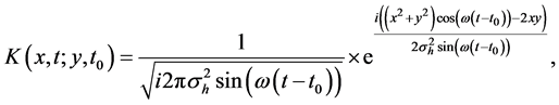 (2)
(2)
with![]() . The KD beam-splitter is realized with an impulse application of a periodic potential
. The KD beam-splitter is realized with an impulse application of a periodic potential![]() , where
, where ![]() is the strength of the pulse,
is the strength of the pulse, ![]() is the atomic recoil energy and
is the atomic recoil energy and![]() . In the Raman-Nath limit [10] [26] [27] , the duration of the pulse is short enough to not affect the atomic density but to only change the phase of the initial wave-function
. In the Raman-Nath limit [10] [26] [27] , the duration of the pulse is short enough to not affect the atomic density but to only change the phase of the initial wave-function ![]() as
as
![]() (3)
(3)
where we have used the Bessel generating function ![]() [28] and
[28] and
![]() . The Raman-Nath limit has been experimentally demonstrated in [21] [29] . Equation (3) shows that the KD beam-splitter creates
. The Raman-Nath limit has been experimentally demonstrated in [21] [29] . Equation (3) shows that the KD beam-splitter creates ![]() copies of the initial state, each with amplitude
copies of the initial state, each with amplitude ![]() and an additional momentum
and an additional momentum![]() .
.
After the application of the first KD, the wave-packets are coherently driven by the harmonic trap and recombined after a time![]() . At this time, the propagator
. At this time, the propagator ![]() in Equation (2) is simply given by
in Equation (2) is simply given by
![]() (4)
(4)
Furthermore, in presence of an external field, each spatial mode created by the KD beam splitter gains during the time ![]() a phase shift
a phase shift ![]() with respect to its neighbour’s modes. Right before the application of a second KD pulse, at time
with respect to its neighbour’s modes. Right before the application of a second KD pulse, at time![]() , the wave function is
, the wave function is
![]() (5)
(5)
After iterating a number of times n the sequence of KD pulses and phase shift accumulations, the wave function at ![]() becomes
becomes
![]() (6)
(6)
where
![]()
and ![]() is the integer part of
is the integer part of![]() . For odd n we have
. For odd n we have
![]()
while for even n we have
![]()
After n iterations, a last KD pulse is applied at the time ![]() providing
providing
![]() (7)
(7)
The wave packets gain their maximum spatial separation after a further ![]() evolution in the harmonic trap.
evolution in the harmonic trap.
Eventually, the wave function at the final time ![]() right before measurement is
right before measurement is
![]() (8)
(8)
where
![]() (9)
(9)
and
![]() (10)
(10)
with![]() ,
, ![]() or 0 for odd or even n, respectively,
or 0 for odd or even n, respectively, ![]() and
and
![]()
![]()
In the limit if zero overlap between the various wave packets in Equation (8),
![]() (11)
(11)
the density function at the measurement time ![]() simply becomes
simply becomes
![]() (12)
(12)
Equation (12) shows that there are ![]() momentum modes created by the n applications of the KD pulses. This can of course be helpful if only weak KD pulses can be experimentally implemented.
momentum modes created by the n applications of the KD pulses. This can of course be helpful if only weak KD pulses can be experimentally implemented.
In the limit of a large number ![]() of independent interferometric measurements, the phase estimation sensitivity saturates the Cramér-Rao [30] lower bound
of independent interferometric measurements, the phase estimation sensitivity saturates the Cramér-Rao [30] lower bound
![]() (13)
(13)
where N is the number of uncorrelated atoms. F denotes the Fisher information calculated from the particle density at the measurement time
![]() (14)
(14)
With Equation (12), Equation (14) becomes
![]() (15)
(15)
(see Appendix). We finally obtain
![]() (16)
(16)
where
![]()
![]()
Notice that even in the case of a odd value of n, with![]() ,
,![]() . Therefore, for an even n or an odd
. Therefore, for an even n or an odd![]() , the phase estimation uncertainty of our interferometer becomes:
, the phase estimation uncertainty of our interferometer becomes:
![]() (17)
(17)
which can also be written as
![]() (18)
(18)
since the total number of modes is![]() . As expected on a general ground from the theory of multimode interferometry [31] , the sensitivity scales linearly with the number of momentum modes which have been significantly populated after KD beam splitters. The populations of higher diffraction orders vanish exponentially [10] .
. As expected on a general ground from the theory of multimode interferometry [31] , the sensitivity scales linearly with the number of momentum modes which have been significantly populated after KD beam splitters. The populations of higher diffraction orders vanish exponentially [10] .
We remark here the important condition of non overlap of the wave packets corresponding to the different momentum modes at the time of measurement, Equation (11). A further interesting point is that Equation (18) is independent from the temperature of the atoms as long as their de Broglie wavelength remains larger than the internal spatial separation of the periodic potential creating the Kapitza-Dirac pulse. We will show this in the following Sections by considering as a specific application the interferometric estimation of the gravitational constant.
4. Estimation of the Gravitational Acceleration Constant g
We now investigate the KD interferometer theory to estimate the gravity constant g. The evolution of the initial state ![]() is influenced by the combined action of the harmonic confinement
is influenced by the combined action of the harmonic confinement![]() , the gravitational field
, the gravitational field ![]() and the KD beam splitters. The goal is to estimate the value of the acceleration constant g. As explained in the previous Section, the phase shift
and the KD beam splitters. The goal is to estimate the value of the acceleration constant g. As explained in the previous Section, the phase shift ![]() arises from the external gravitational field acting during the phase accumulation period (until
arises from the external gravitational field acting during the phase accumulation period (until![]() ). We may engineer our Hamiltonian to switch on/off the gravity after the first beam splitter by modifying the frequency of the harmonic trap by
). We may engineer our Hamiltonian to switch on/off the gravity after the first beam splitter by modifying the frequency of the harmonic trap by![]() , where
, where ![]() are the trap frequencies before and after the KD, respectively. We finally generalize our results by considering an atomic gas in thermal equilibrium at a finite temperature
are the trap frequencies before and after the KD, respectively. We finally generalize our results by considering an atomic gas in thermal equilibrium at a finite temperature![]() .
.
To take in account the effect of the gravitational force on the dynamical evolution of the trapped atom states, we need to include in the free propagator ![]() Equation (2) the linear gravitational field [25]
Equation (2) the linear gravitational field [25]
![]() (19)
(19)
where ![]() and
and ![]() with
with![]() . After the application of the first KD, the states are coherently driven by the harmonic trap and the external gravitational field. At the time
. After the application of the first KD, the states are coherently driven by the harmonic trap and the external gravitational field. At the time![]() , each spatial modes, created by KD pulse, are recombined and the wave function becomes
, each spatial modes, created by KD pulse, are recombined and the wave function becomes
![]() (20)
(20)
since the quantum propagator undergone with gravity field is reduced to
![]() (21)
(21)
As expected, each spatial mode gains its phase shift ![]() with respect to its neighbour’s modes at time
with respect to its neighbour’s modes at time ![]() due to action of the external gravity field after the first KD pulse. A straightforward (slightly tedious) calculation provides the wave function at
due to action of the external gravity field after the first KD pulse. A straightforward (slightly tedious) calculation provides the wave function at ![]()
![]() (22)
(22)
where ![]() for even n and
for even n and ![]() for odd n. The function
for odd n. The function ![]() also depends on the of n: for odd n we have
also depends on the of n: for odd n we have
![]()
and for even n
![]()
The last KD pulse is applied on the wave function Equation (22) at time![]() , to mix and therefore spatially separate the modes for the final density profile measurement
, to mix and therefore spatially separate the modes for the final density profile measurement
![]() (23)
(23)
Firstly, we consider the case without the gravity field. Then at the time ![]() , the wave function is
, the wave function is
![]() (24)
(24)
where ![]() and for n even (odd)
and for n even (odd) ![]() (
(![]() ).
).![]() is defined by
is defined by
![]() (25)
(25)
and ![]() be found by replacing integral function
be found by replacing integral function ![]() as
as ![]() in Equation (10). Secondly, with gravity field, the wave function under quantum propagator with gravity field
in Equation (10). Secondly, with gravity field, the wave function under quantum propagator with gravity field
![]() (26)
(26)
where ![]() is defined by Equation (9), can be expressed as
is defined by Equation (9), can be expressed as
![]() (27)
(27)
where ![]() is defined by Equation (24) and
is defined by Equation (24) and
![]()
![]()
Except the phase difference between Equation (24) and Equation (27), a constant difference d is found in the centre position of each sub-wave packets induced by the gravity field. In the case of “no-overlap” condition (Equation (11)), which is satisfied when the width of the initial wave packet is much larger than the interwell distance of the KD optical lattice (![]() ), the final density function becomes
), the final density function becomes
![]() (28)
(28)
from Equation (24) or
![]() (29)
(29)
from Equations ((27), (12) and (28)) show that the information on the estimated values of ![]() and g are mainly (or entirely) contained in the weights
and g are mainly (or entirely) contained in the weights![]() , depending on the final evolution during the measurement period. A small part of the information is involved in the center of sub-wave packets for half gravity evolution (Equation (29)).
, depending on the final evolution during the measurement period. A small part of the information is involved in the center of sub-wave packets for half gravity evolution (Equation (29)).
We now consider an atomic gas at finite temperature T. To get some simple insight on the physics of the problem, we consider the system as made by a swarm of minimum uncertainty Gaussian wave packets
![]() (30)
(30)
where the initial wave packet width ![]() is equal to the thermal de Broglie wavelength
is equal to the thermal de Broglie wavelength ![]() while the initial average coordinates
while the initial average coordinates ![]() and momentum
and momentum ![]() are distributed according to the Boltzmann-Maxwell distribution
are distributed according to the Boltzmann-Maxwell distribution
![]() (31)
(31)
Each wav packet evolves driven by the propagators calculated in the previous Section:
![]() (32)
(32)
and
![]() (33)
(33)
where ![]() for odd n and
for odd n and ![]() for even n. Replacing in Equation (31), we find that the density distribution at the output of the interferometer is
for even n. Replacing in Equation (31), we find that the density distribution at the output of the interferometer is
![]() (34)
(34)
where ![]() is the normalization constant and
is the normalization constant and
![]() (35)
(35)
![]() (36)
(36)
It is interesting to note that![]() . In the case of
. In the case of![]() , only the terms with
, only the terms with ![]() in Equation (34) are important and the density profile at the final time reduces to a sum of weighted Gaussians of width
in Equation (34) are important and the density profile at the final time reduces to a sum of weighted Gaussians of width![]() :
:
![]() (37)
(37)
or
![]() (38)
(38)
Notice that the value of the gravitational constant g is only contained in the weights of the modes.
The requirement is that sub-wave packets in Equation (37) are spatially separated, which means![]() . Considering Equation (35), we have
. Considering Equation (35), we have
![]() (39)
(39)
which means
![]() (40)
(40)
As expected, the spatial separation condition in Equation (37) ![]() is equivalents to
is equivalents to![]() . This means that the initial wave packets width (the thermal de Boglie wavelength) should be much larger than the internal distance of the KD potential. This is consistent with Equation (11). The important result is that as long as this condition is satisfied, the sensitivity does not depend on the temperature.
. This means that the initial wave packets width (the thermal de Boglie wavelength) should be much larger than the internal distance of the KD potential. This is consistent with Equation (11). The important result is that as long as this condition is satisfied, the sensitivity does not depend on the temperature.
Substituting the density function Equation (37) at the measurement time ![]() into Fisher information Equation (14), we obtain
into Fisher information Equation (14), we obtain
![]() (41)
(41)
The Fisher information for our system depends on the temperature, initial density profile, the interferometer transformation, and the choice of the observable that, here, is the spatial position of atoms. In this case, the estimator can simply be a fit of the final density profile. However, the same results would be obtained by choosing as observable, the number of particles in each Gassian spatial mode. Since the initial state is made of uncorrelated atoms, there is no need to measure correlations between the modes in order to saturate the Cramér-Rao lower bound Equation (13) at the optimal value of the value phase shift.
Before proceeding to discuss the finite temperature case, we calculate the highest sensitivity of the unbiased estimation of parameter g, which is guaranteed by the no-overlap condition![]() .
.
In the limit![]() , the Fisher information can be calculated analytically
, the Fisher information can be calculated analytically
![]() (42)
(42)
where ![]() for even n and
for even n and ![]() for odd n, with
for odd n, with ![]() in the limit
in the limit![]() . Finally, the Cramér-Rao lower bound Equation (13) becomes
. Finally, the Cramér-Rao lower bound Equation (13) becomes
![]() (43)
(43)
The Equation (43) can be rewritten as
![]() (44)
(44)
where![]() .
.
If the gravity field is witched on in the last KD pulse, the density profile at final time is described by Equation (38). In this case, there is a further contribution to the Fisher Equation (42) from the shift on the center of sub-wave packets and we have
![]() (45)
(45)
5. Sensitivity
We now estimate the expected sensitivity under realistic experiment conditions. We consider 105 88Sr atoms trapped in an harmonic trap having ![]() and a Kapitza-Dirac periodic potential with
and a Kapitza-Dirac periodic potential with ![]() [21] , recoil energy
[21] , recoil energy ![]() and KD pulses applied for a time
and KD pulses applied for a time![]() .
.
With a strength of the KD potential ![]() [21] , a single pulse creates ~9 modes which provide a sensitivity with a single measurement shot and a phase accumulation time of 0.1 seconds,
[21] , a single pulse creates ~9 modes which provide a sensitivity with a single measurement shot and a phase accumulation time of 0.1 seconds,![]() . This sensitivity increases as
. This sensitivity increases as![]() , see Equation (43), after n pulses and phase accumulation time up to
, see Equation (43), after n pulses and phase accumulation time up to ![]() seconds. Under these conditions, the maximum length spanned by the 88Sr atoms is also increased from
seconds. Under these conditions, the maximum length spanned by the 88Sr atoms is also increased from ![]() to
to![]() , see the black lines in Figure 3. In practice the sensitivity is limited by the effective length of the harmonic confinement. With current technologies using magnetic traps, the largest spatial separation L could be pushed up to a few millimeters.
, see the black lines in Figure 3. In practice the sensitivity is limited by the effective length of the harmonic confinement. With current technologies using magnetic traps, the largest spatial separation L could be pushed up to a few millimeters.
Since the thermal de Broglie wavelength decreases when increasing the temperature, the no-overlap condition Equation (11) breaks down at![]() . In Figure 2, we plot the normalised sensitivity as a function of the temperature. The time-independent sensitivity is found for various numbers of KD pulses. Once the temperature is increased up to the crossover value
. In Figure 2, we plot the normalised sensitivity as a function of the temperature. The time-independent sensitivity is found for various numbers of KD pulses. Once the temperature is increased up to the crossover value![]() , the sensitivity is drastically reduced see Figure 2. When
, the sensitivity is drastically reduced see Figure 2. When![]() , the wave packets are spatially addressable (see dark and blue lines in Figure 3). When
, the wave packets are spatially addressable (see dark and blue lines in Figure 3). When![]() , the distinguishability of the wave packets decreases (red lines in Figure 3) and the uncertainty in the phase estimation increases as
, the distinguishability of the wave packets decreases (red lines in Figure 3) and the uncertainty in the phase estimation increases as ![]() for
for![]() .
.
![]()
Figure 2. (color-online) Normalized phase estimation sensitivity as a function of the temperature for even and odd n.
![]()
Figure 3. (color-online) Density profiles of the output wave function of Figure 2. The dark line, blue line and red line show temperatures below, equal and above the crossover temperature![]() .
.
As a comparison with current atom interferometers, we calculate the sensitivity obtained from a simple interference pattern observed after a free expansion of an initial atom clouds relevant, for instance, when measuring the gravitational constant g using Bloch oscillations [12] [13] [14] . As shown in [32] , the momentum distribution is expressed as
![]() (46)
(46)
where ![]() is the wave length of the laser. A is a normalization factor and j denotes the lattice site and
is the wave length of the laser. A is a normalization factor and j denotes the lattice site and ![]() is the phase difference between lattice site. Since the finite size of the initial cold atomic cloud, there is only a finite number of terms in Equation (46) which contribute to the sum. We therefore have
is the phase difference between lattice site. Since the finite size of the initial cold atomic cloud, there is only a finite number of terms in Equation (46) which contribute to the sum. We therefore have
![]() (47)
(47)
where ![]() is the maximum numbers of the lattice occupied by the initial atom gases. In Equation (46), each point
is the maximum numbers of the lattice occupied by the initial atom gases. In Equation (46), each point ![]() has a Gaussian momentum distribution. Therefore, we obtain
has a Gaussian momentum distribution. Therefore, we obtain
![]() (48)
(48)
where![]() . Considering the experimental situations in [12] [13] [14] ,
. Considering the experimental situations in [12] [13] [14] , ![]() , we arrive at
, we arrive at
![]() (49)
(49)
where ![]() is the interaction time of the neighbour cold atom under the gravity-like force. Therefore it could be approximate as the tunnelling time
is the interaction time of the neighbour cold atom under the gravity-like force. Therefore it could be approximate as the tunnelling time ![]() s in [13] . With the Cramér-Rao lower bound Equation (13), we have
s in [13] . With the Cramér-Rao lower bound Equation (13), we have
![]() (50)
(50)
where we have estimated the maximum occupied lattice sites by![]() . Therefore, the sensitivity is
. Therefore, the sensitivity is
![]() (51)
(51)
Considering the sensitivity for a single Kaptiza-Dirac pulse with Equation (51), we can reach a sensitivity larger than 3 order of magnitude that the sensitivity obtained in an interference pattern. The reason is that the KD pulses can create several wave packets spanning a distance![]() , which can be quite a bit larger than the typical distances between the wave packets created in far field expansion measurements. In this case, the theoretical gain provided by Equation (43) is proportional to
, which can be quite a bit larger than the typical distances between the wave packets created in far field expansion measurements. In this case, the theoretical gain provided by Equation (43) is proportional to![]() , which can be ~103 with only once KD pulse and typical values of the experimental parameters. A further advantage is that such high sensitivity interferometry can be realised with a compact experimental setup.
, which can be ~103 with only once KD pulse and typical values of the experimental parameters. A further advantage is that such high sensitivity interferometry can be realised with a compact experimental setup.
6. Noise and Decoherence
We now consider the effects of noise and imperfections on the sensitivity of the interferometer. We mainly consider two kinds of perturbations, which may arise from the experimental realization of the interferometry. The first one is the effect of the anharmonicity, described by a position dependent random perturbation, and the second one the effect of a shift in position between different sequences of the KD pulses.
The effect of anharmonicity is investigated by numerically simulating the interferometric sequences with the following potential
![]() (52)
(52)
where![]() .
. ![]() is the strength of a position dependent random perturbation
is the strength of a position dependent random perturbation ![]() having values
having values![]() . We take as length unit of the harmonic trap
. We take as length unit of the harmonic trap ![]() and as time unit the inverse of the trap frequency
and as time unit the inverse of the trap frequency![]() . The strength of the external gravity-like potential is described by a dimensionless parameter
. The strength of the external gravity-like potential is described by a dimensionless parameter![]() , then
, then![]() . To simplify the simulation, in the following we only consider a single KD pulse.
. To simplify the simulation, in the following we only consider a single KD pulse.
Starting with the ground state of the harmonic trap![]() , the time dependent wave functions can be found by operator splitting method [33] with
, the time dependent wave functions can be found by operator splitting method [33] with![]() . Using
. Using ![]() groups of random numbers, we generate
groups of random numbers, we generate ![]() densities at the measurement time. Then,
densities at the measurement time. Then,
the average density ![]() is used for calculating Fisher
is used for calculating Fisher
information ![]() for given
for given![]() . Here, we use the Equation (53) to get the derivative for
. Here, we use the Equation (53) to get the derivative for ![]() and
and ![]()
![]() (53)
(53)
Due to the perturbation potential![]() , the sub-wave packets are driven back to their initial position with a incoherent phase at
, the sub-wave packets are driven back to their initial position with a incoherent phase at ![]() and the total density profile could be dramatically destructed. It is interesting to note that the KD pulses still do a quite good job and that completed spatially separated wave packets with momentum
and the total density profile could be dramatically destructed. It is interesting to note that the KD pulses still do a quite good job and that completed spatially separated wave packets with momentum ![]() can be found at the measurement time
can be found at the measurement time![]() , see Figure 4. When increasing
, see Figure 4. When increasing![]() , the visibility of the wave packets decreases compared with the ideal case (Black line, without
, the visibility of the wave packets decreases compared with the ideal case (Black line, without![]() ). This definitely makes a impact on the sensitivity, which can be found by calculating the Fisher information
). This definitely makes a impact on the sensitivity, which can be found by calculating the Fisher information ![]() through
through![]() . The results have been presented in Figure 5. Generally speaking, a strong perturbation of the harmonic potential decreases dramatically, see Figure 5(b), while, for
. The results have been presented in Figure 5. Generally speaking, a strong perturbation of the harmonic potential decreases dramatically, see Figure 5(b), while, for ![]() it is still possible to obtain a sensitivity comparable with the ideal case.
it is still possible to obtain a sensitivity comparable with the ideal case.
A shift of the optical lattice with respect to the harmonic trap ![]() is further possible reason for a decreased sensitivity. Assuming a off center shift of two consecu-
is further possible reason for a decreased sensitivity. Assuming a off center shift of two consecu-
tive KD pulses![]() , the wave function at
, the wave function at ![]() after the second KD is
after the second KD is
![]() (54)
(54)
where![]() . To get this result we have considered the properties of Bessel generating function [28] .
. To get this result we have considered the properties of Bessel generating function [28] .
![]() (55)
(55)
where![]() . Equation (55) shows that the effect of off-center shift
. Equation (55) shows that the effect of off-center shift
makes only an phase shifts for each sub-wave packets. Therefore, the non-overlap condition Equation (11) does not have any modification even after considering the off-center shift In this case, the final density profiles is
![]() (56)
(56)
Equation (56) shows that the center shifts could induce a fluctuation by ![]() around the estimated value of d. If those off-center shifts are coming from some external noise, then it may do not play crucial effect on the value of
around the estimated value of d. If those off-center shifts are coming from some external noise, then it may do not play crucial effect on the value of![]() . Therefore, it does have small effect on Fisher information, by
. Therefore, it does have small effect on Fisher information, by
![]() (57)
(57)
7. Conclusion
During the last few decades, matter-wave interferometry has been successfully extended to the domain of atoms and molecules. Most current interferometric protocols for the measurement of gravity or inertial forces are based on the manipulation of free falling atoms realizing Mach-Zehnder like configurations. Here we propose an atomic multimode interferometer with atoms trapped in a harmonic potential and where the multi beam-splitter operation are implemented with Kapitza-Dirac pulses. The mirror operations are performed by the harmonic trap which coherently drives a tunable number of spatially addressable atomic beams. All interferometer processes, including splitting, phase accumulation and reflection are performed and completed within the harmonic trap. Therefore, all trapped atoms contribute to the sensitivity. We have applied our scheme to the estimation of the gravitational constant and estimate, with realistic experimental parameters, a sensitivity of 10−9, significantly exceeding the sensitivity of current interferometric protocols.
Acknowledgements
Our work is supported by the National Science Foundation of China (No. 11374197), PCSIRT (No. IRT13076), the National Science Foundation of China (No.11504215).
Appendix
Appendix A
To obtain Equation (15), we have considered the Bessel functions identity
![]()
With this we have
![]() (58)
(58)
where one more identity
![]() (59)
(59)
has been used to obtain
![]() (60)
(60)
Appendix B
For Equation (45), Using the Equation (41) and Equation (29), we obtain
![]() (61)
(61)
By using the initial state
![]() (62)
(62)
we get
![]() (63)
(63)
where ![]() for even n, but
for even n, but ![]() for odd n. So
for odd n. So
![]() (64)
(64)
The second step uses the “no-overlap” condition by changing ![]() to
to ![]() in Equation (11).
in Equation (11).
![]()
Submit or recommend next manuscript to SCIRP and we will provide best service for you:
Accepting pre-submission inquiries through Email, Facebook, LinkedIn, Twitter, etc.
A wide selection of journals (inclusive of 9 subjects, more than 200 journals)
Providing 24-hour high-quality service
User-friendly online submission system
Fair and swift peer-review system
Efficient typesetting and proofreading procedure
Display of the result of downloads and visits, as well as the number of cited articles
Maximum dissemination of your research work
Submit your manuscript at: http://papersubmission.scirp.org/
Or contact jmp@scirp.org