The Estimation of the Error at Richardson’s Extrapolation and the Numerical Solution of Integral Equations of the Second Kind

Igor Petrovich Dobrovolsky

Institute of Physics of the Earth, Russian Academy of Sciences, Moscow, Russia.

DOI: 10.4236/oalib.1102051                

Abstract

The mode of definition of the error at polynomial Richardson’s extrapolation is described. Along with the table of extrapolations the new magnitudes reflecting expediency and efficiency of extrapolation are entered. On concrete examples it is shown that application of Richardson’s extrapolation to a solution of integral equations has appeared rather effective and gives a solution with a high exactitude. Application of formulas of interpolation leads to a solution in the analytical aspect.

Keywords

The Trapezoidal Rule, Continued Fraction, The Index of Richardson’s Extrapolation

Subject Areas: Geology, Geophysics

1. Introduction

Numerical methods of the approached solution are attractive by the universality. In numerical methods three problems are put: obtaining enough exact solutions, accuracy control and algorithmic simplicity of procedures. Richardson’s extrapolation solves these problems. The first work of this theme was [1] . Since then many works (for example [2] ) are published and there is no necessity to do one more review. However, it is impossible to consider a theme exhausted. For example, in full enough handbook [3] , there is no even a mention of application of Richardson’s extrapolation to a solution of integral equations.

The purpose of this paper is to construct procedure of an estimation of an error at Richardson’s extrapolation and to apply it to a numerical solution of integral equations of the second kind of Volterra and Fredholm.

2. About Polynomial Richardson’s Extrapolation

We shall briefly remind an essence of Richardson’s extrapolation.

There are many problems from different sections of mathematics in which the difference between exact and approached by solutions (an error of calculation of r) at sufficient smoothness of functions of a problem has expansion

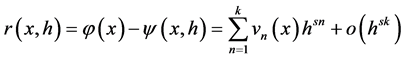. (2.1)

Magnitude h is usually a grid step.

We shall designate the approached solution as

. (2.2)

is called as extrapolation of the zero order.

Extrapolation of the 1-st order is obtained by elimination of the first term of expansion (2.1) by a linear combination of extrapolations of the zero order. Extrapolation of the j-st order is calculated on the recurrence formula

(2.3)

where usually is accepted.

In the end a table of extrapolations is obtained

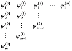. (2.4)

3. The Analysis of the Table of Extrapolations in Special Case

If magnitude h forms a geometrical progression

(3.1)

that (2.3) receives an aspect

. (3.2)

In this case from (3.2) and (2.1) we have

(3.3)

where lack of the top sign at the sum means that the remainder term is included in this sum.

We will name as the index of extrapolation ratio

. (3.4)

Extrapolation improves an exactitude in comparison with when.

From (3.3) follows

(3.5)

where.

Because we have an obvious relation

. (3.6)

By means of the Formula (3.5) table is created.

Obviously, at a diminution h there occurs such moment when terms in expansion (3.3) start to decrease monotonically. We name this mode regular. If extrapolation becomes on a regular mode, the first term should bring the basic contribution in expansion (3.5). Then the relation should be observed

. (3.7)

And on the contrary: if the relation (3.7) is observed, we have a regular mode. Magnitude is almost constant in a table column. By means of the Formula (3.7) table is created.

Let’s enter magnitude

(3.8)

and we shall define its meaning.

From (3.8), we have

. (3.9)

Substituting (3.9) in (3.2) we receive

. (3.10)

From (3.4), (3.6), (3.9) and (3.10) , we have

. (3.11)

Therefore, is estimation the index of extrapolation. By means of the Formula (3.8) table is created.

By Formulas (3.6), (3.7), (3.11) and assumption the error estimation is

. (3.12)

Starting from row (3.5) and definition (3.8), it is possible to establish that there is the expansion for

(3.13)

where the first item has a basic meaning in a regular mode.

Then from (3.13) we receive the relation

at (3.14)

on all table irrespective of an index j.

4. The Numerical Solution of Integral Equation of Volterra

Let’s consider integral equation of Volterra of the second kind.

(4.1)

where and.

This equation has an exact solution

. (4.2)

We shall designate the approximate solution of the Equation (4.1) at the calculation of integrals on a trapezoidal rule with extrapolation by.

Procedure of a solution of integral equation of Volterra of the second kind with application of the trapezoidal rule is known (for example [3] ). At the calculation of integrals by the trapezoidal rule s = 2. At q = 2 each previous set of points contains in the subsequent set and it enables application of extrapolation. Then (3.3) receives the form

(4.3)

and (3.2) receives the form

. (4.4)

It is sometimes more convenient to use “direct” formulas

(4.5)

which come out by sequential application of the Formula (4.4).

Let’s consider (4.1) on a piece x = 0 ÷ 2.5 with step. Below tables of extrapolations and other magnitudes according to formulas of the previous section are reduced. Calculations were made with 15-th significant digits, but for convenience of reading in tables of number are approximated.

By means of the Formula (3.5) table is created.

By means of the Formula (3.7) table is created.

By means of the Formula (3.8) table is created.

The analysis of tables leads to the important conclusions. From Table 1 and Table 2 follows that is the most exact value. It is visible from Table 3 that the Formula (3.7) is satisfactorily satisfied. From Table 4 follows,

Table 1. Table of extrapolation in the point x = 2.5. The exact magnitude is shown by bold type.

Table 2. The table of.

Table 3. The table of.

Table 4. The table of.

that depends from j a little at everyone i. Now it is possible to make an estimation of the error of at x = 2.5. From (3.12) we have

. (4.6)

The true error is.

We have received the precision solution in isolated points. It is interesting to find good interpolation function and to receive a solution in the analytical form. Let’s make uniform set from with the step 0.1 (26 points). Interpolation by continuous fractions (the command Thiele Interpolation in the package Curve Fitting of the program Maple) was better than interpolation by cubic splines. Interpolation by continuous fractions we shall

designate and serves as control value. These results are presented in Table 5.

The Equation (4.1) for area can be written down in the form.

. (4.7)

The Equation (4.7) defines the solution at if function is known at.

5. The Numerical Solution of Integral Equation of Fredholm

The equation is considered

(5.1)

which has the exact solution.

Procedure of a solution of integral equation of Fredholm of the second kind with application of the trapezoidal

Table 5. Interpolation and exact solution. At x = 2.488 interpolation has the largest error.

rule is also known (for example [3] ). We keep designations of the previous section. We shall produce tables (also with a rounding) without explanations as the analysis of tables is invariable (Tables 6-9).

From (3.12) we have the estimation of the error of. The true error is.

The remark. Trapezoidal rule is the scheme of 2-nd order of exactitude and s = 2 in expansions (2.1) and (3.3). For a calculation of interpolations of zero order it is possible to use Simpson’s formula (the formula of 4-th order of exactitude). For Simpson’s formula expansion on even degrees is kept, but in (2.1) and (3.3) the first term vanishes. Formally it means: in (2.1) and (3.3) we do replacement, but it is necessary to preserve indexes of terms and. Formulas (2.1) and (3.3) get the form (at s = 2)

(5.2)

and

. (5.3)

If to begin calculations from Simpson’s formula then in the formula (3.2) it is necessary to replace; but it does not concern magnitudes as we keep the indexing the order of extrapolation. The formula (3.2) receives the form

(5.4)

and “direct” formulas receive the kind

. (5.5)

The important note: by means of the formula (3.2), it is easy to establish that Simpson’s formula is extrapolation of 1-st order of a trapezoidal rule and there is no real necessity to use Simpson’s formula. Let’s remind that application of any schemes of a high exactitude demands high smoothness of functions.

6. Conclusion

Trapezoidal rule with Richardson’s extrapolation is the effective method of a solution of integral equations of the second kind, and with application of interpolation we receive a solution in an analytical aspect. In this case the table of extrapolations enables to make a good estimation of an error of solution. The received solution possesses a high exactitude and can be the standard for other methods of a solution of the equation.

Table 6. Table of extrapolation in the point x = 1. The exact magnitude is shown by bold type.

Table 7. The table of.

Table 8. The table of.

Table 9. The table of.

Conflicts of Interest

The authors declare no conflicts of interest.

References

[1]	Richardson, L.F. (1911) The Approximate Arithmetical Solution by Finite Differences of Physical Problems Involving Differential Equations with an Application to the Stress in a Masonry Dam. Philosophical Transactions of the Royal Society of London. Series A, 210, 307-357.
[2]	Stetter, H.J. (1973) Analysis of Discretization Methods for Ordinary Differential Equations. (Springer Tracts, Vol. 23). Springer, Berlin, Heidelberg and New York.
[3]	Polyanin, A.D. and Manzhirov, A.V. (2008) Handbook of Integral Equations. Chapman & Hall/CRC Press, Boca Raton and London. http://dx.doi.org/10.1201/9781420010558