On the Approximation of Maximum Deviation Spline Estimation of the Probability Density Gaussian Process

Mukhammadjon S. Muminov¹, Kholiqjon S. Soatov²

¹Institute of Mathematics, National University of Uzbekistan, Tashkent, Uzbekistan.
²Tashkent University of Information Technologies, Tashkent, Uzbekistan.

DOI: 10.4236/ojs.2015.54034                

Abstract

In the paper, the deviation of the spline estimator for the unknown probability density is approximated with the Gauss process. It is also found zeros for the infimum of variance of the derivation from the approximating process.

Keywords

Spline-Estimator, Distribution Function, Gauss Process

1. Introduction

The present work is a continuation of the work [1] , that’s why we use notations admitted in it. We shall not turn our attention to more detailed review because it is given [1] .

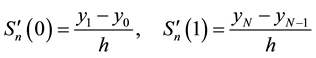
Let be a simple sample from the parent population with the probability density concentrated and continuous on the segment. Let be a cubic spline interpolating values at the points, with the boundary conditions

where, , , as.

Remind that

,

,

,

where, is the kernel of the spline, see [1] , is a sequence

of Wiener processes.

Denote by the distribution function of the random variable

,

and by the distribution functions of the random variable

,

where

. (1)

In the second section of the work, Theorem 2 and 3 are proven:

and

And it is also stated (Theorem 5) that

2. Formulation and Proof the of Main Results

It holds the following

Theorem 1. Let and be random variables, in addition for some,. Then for any x

.

The proof of this statement is easy, therefore we omit it.

Theorems 2 and Theorem 3 will be proved by the mthods given in [2] .

Theorem 2. Let, , and there exist a constant such that

. (2)

Then under our assumption a) and b) concerning, there exists a constant such that for sufficiently large n

.

Proof. By the main Theorem from [1] ,

, (3)

and for any

. (4)

Set.

Theorem 2 follows now from Theorem 1, relations (2) from [1] , inequalities (3) and (4), and the fact that the

random variables and have the same distribution.

Theorem 3. If conditions of Theorem 2 hold and, then for sufficiently large n

,

where is a constant, , is defined in (2).

Proof. From the interpolation condition

we have

.

One can easily note that is a cubical spline interpolating of

,

in the points of interpolation,. On the other hand. By Theorem 9 from the monograph [3] we get

, (5)

where

.

The relation (5) implies that for arbitrary

It remains to choose and using Theorem 1 [1] . Theorem 3 is proved.

Relations imply

Theorem 4. First order mean square derivations of the Gauss process are continuous in [0, 1], and second order mean square derivations do not have discontinuity in the points of the spline interpolation.

Let now be points of the cubical spline interpolation, and be a uniform partition of the interval [0, 1]. Is is valid the following

Theorem 5. 1) The variance of mean square derivations of the Gauss process

vanishes in the intervals and at the points and, respectively;

2) If the variance vanishes also in intervals, then there will be not more than two roots in each interval.

Proof. At the beginning of the proof of the theorem, we proceed as in [2] . Let. Then using the relation ([4] , p. 28)

we get for

(6)

Substituting into (6)

and taking into account that, we obtain

or

We find analogously

and also

Generalizing the obtained results, we have

Denote. The equality

implies

On the other hand,

where

.

Obviously,. The point will be a solution of the equation

. Recall that. Like the case of, we can act analogously in the case of,

i.e. at, when.

The first part of Theorem 5 is proved.

Let pass to the proof of the second part. Both in the case of, i.e. when, , and in the case of, the equality

is valid for,.

The explicit form of is given in Muminov (1987), and it is very cumbersome.

Note, in this case also.

One can easily see that is the sum of second powers of quadratic trinomials with respect to, and it has not more than two real roots if they exist in [0, 1].

The first part of Theorem 5 is proved.

At last, Theorems 2 and 3 imply that limit distributions of the random variables and

coincide. However, the Gauss process does not have second order mean square derivatives in the inter-

polation points for the spline, and. Therefore one can not apply results of the works [5] -[7]

to investigate the distribution of the maximum of. This deficiency has been removed in [8] .

NOTES

^*Corresponding author.

Conflicts of Interest

The authors declare no conflicts of interest.

References

[1]	Muminov, M.S. and Soatov, Kh. (2011) A Note on Spline Estimator of Unknown Probability Density Function. Open Journal of Statistics, 157-160. http://dx.doi.org/10.4236/ojs.2011.13019
[2]	Khashimov, Sh.A. and Muminov, M.S. (1987) The Limit Distribution of the Maximal Deviation of a Spline Estimate of a Probability Density. Journal of Mathematical Sciences, 38, 2411-2421.
[3]	Stechkin, S.B. and Subbotin, Yu.N. (1976) Splines in Computational Mathematics. Nauka, Moscow, 272p.
[4]	Hardy G.G., Littlewood, J.E. and Polio, G. (1948) Inequalities. Moscow. IL, 456 p. http://dx.doi.org/10.1007/BF01095085
[5]	Berman, S.M. (1974) Sojourns and Extremes of Gaussian Processes. Annals of Probability, 2, 999-1026. http://dx.doi.org/10.1214/aop/1176996495
[6]	Rudzkis, R.O. (1985) Probability of the Large Outlier of Nonstationary Gaussian Process. Lit. Math. Sb., XXV, 143-154.
[7]	Azais, J.-M. and Wschebor, M. (2009) Level Sets and Extrema of Random Processes and Fields, Wiley, Hoboken, 290p.
[8]	Muminov, M.S. (2010) On Approximation of the Probability of the Large Outlier of Nonstationary Gauss Process. Siberian Mathematical Journal, 51, 144-161. http://dx.doi.org/10.1007/s11202-010-0015-6