An Alternative Manifold for Cosmology Using Seifert Fibered and Hyperbolic Spaces ()
1. Introduction
In his field equations, Einstein just provided a compact mathematical tool that made it possible to develop a theory to describe the general configuration of matter-energy and space-time for the Universe. Nevertheless, the questions related to the global shape of space and, in particular, its finite or infinite extension, cannot be fully answered by the General Relativity (a local physical theory). That is why, the use of topology (a global mathematical theory) is necessary to construct a new manifold which could answer some of those questions. Accordingly, many topological “alternatives” of three-dimensional spaces can thus be used to build such cosmological universe models.
The investigation of topological changes may bring a new approach to studying the early cosmology of the universe [1] [2] . The problem of changing topology has been discussed from different points of view in both classical and quantum gravity [3] [4] . In addition, Gauge theory [5] provides an alternative to solve some problems that general relativity can not.
Efremov [6] proposed a manifold which admits 3-dimensional sections of Euclidean space-time cobordisms describing topology changes. In this work we take the Seifert Fibered Spaces represented by homologic spheres and we improve the idea of Efremov [6] [7] and Mitskievich [8] [9] adding hyperbolic cusp spaces. We describe the process of construction of a cosmological model which was used to calculate the coupling constants for fundamental forces as shown in [10] .
We like to point out that our Model of Space-Time does not have singular orbits (those are obtained by factorization with respect to the action group ) because they have been replaced by an hyperbolic manifold. Also, comparing the coupling constants obtained in [6] with the new ones, we can see that the new model has a better fit with those obtained by experiments (see [10] ).
Other works which can be a motivation for using hyperbolic manifolds in physics are: [11] -[14] . However, compared to the work presented here, their approaches are in a very different way because they are limited to a decomposition of Seifert Fibered Spaces and do not use Thurston’s theory for the hyperbolic part.
First we make the decomposition of Seifert Fibered Spaces in prime spaces. This process includes a collection of cuts of a 3-dimensional space  in two parts along 2-dimensional spheres such that the space
  is separated into two parts and neither of these is a 3-dimensional disc. This operation is the inverse of the connected sum. The result of gluing two of 3-dimensional disc to each component of the boundary is to obtain a simpler 3-manifold every time we do the process. Kneser [15] proved that such process is terminated after a finite number of steps. We call prime components of
  as each of the parts that were obtained as a result of this decomposition process. They are solely defined except by homeomorphisms, see [16] .
After that, we involve the decomposition of cuts along a torus. The reverse operation to splice described in [17] , has been discovered by Johanson [18] , Jaco and Shalen [19] . This decomposition along the torus  gives a set of 3-manifolds of which some are Seifert Fibered manifolds and others allow hyperbolic structures. Previous works [6] and [9] , considered a special case. Namely, a 3-dimensional space contains only Seifert fibered spaces represented by homological spheres as parts.
Here, we extend those ideas using Thurston’s conjecture (now proved) [20] -[22] and the work of Jaco [19] [23] and Johanson [18] . This allows glueing a suitable hyperbolic space in Seifert fibered space and taking the Seyfert hyperbolic invariants inside of a hyperbolic space.
2. Introducing Seifert Manifolds and Hyperbolic Spaces
There are several definitions in literature about Seifert Manifolds, here we introduce our own definition of Seifert Manifolds. For hyperbolic spaces we will use Thurston’s theory. Then we will use all those concepts for the construction of a new Manifold representing the cosmological Universe.
Seifert Manifolds
Definition 1. A Seifert Fibered Manifold (SFM) is an orientable three-manifold ,
,  is the collection
  of pairwise disjoint simple closed curves, called fibers, such that for each
  there is a closed neighbourhood
  of
of  which is a solid torus and there is a covering map
  such that:
1)  maps each
  to
to 
2)  are connected.
3) The covering translation group is generated by  where
where

Definition 2. If  is a 3-compact manifold and
  has a Seifert fibration, there is a smooth map
 ,
,  surface with the following property. Each
  has a closed neighbourhood
  such that, the restriction
  to
to  is a diffeomorphism from Seifert fibration to a solid torus. To be more precise, there are relatively prime integers
  and
and , with
  and the diffeomorphisms
  and
and  such that the diagram

is commutative.
Applying the previous definitions. Consider the trivial fibered cylinder , with fibers1
  Identifying cylinder caps and making a rotation
 to a cylinder we obtain a fibered torus, see Figure 1.
The reader can also see [23] .
See Appendix for other useful definitions.
3. Hyperbolic Spaces
In his notes, Thurston [21] describes different models for hyperbolic spaces. However we only take here the upper-half space model. We believe that this particular hyperbolic space has the necessary geometry in order to fulfil the requirements of the physical space. It has itself differents approaches, then in physics we want to be one part flat. In this space inasmuch we can find the ratio of the Euclidean distance. Also has the useful characteristic of having points at infinity.
The upper half-space model (taked from [21] ).
This is closely related to the Poincaré disc model and the southern hemisphere, but it is often more convenient for computation or for constructing graphics. To obtain the upper-half space model, rotate the sphere  in
in  so that the southern hemisphere lies in the half-space
  is
is . Now, the stereographic projection from the top of
  (which is now on the equator) sends the southern hemisphere to the upper half-space in
  As shown in Figure 2.
A hyperbolic line, in the upper half-space, is a circle perpendicular to the bounding plane 
The hyperbolic metric is:

This representation of a hyperbolic space is suitable in physics because we have two things. A manifold with finite volume [24] and the Euclidean image of a hyperbolic object moving toward  has size precisely proportional to the Euclidean distance from
 .
.

Figure 1. (a) Represents the cilinder with fibres and 1(b) is the fibered torus that will appear in our construction.
Here we present the triangulation of the Seifert spheres and hyperbolic spaces in order to preserve the orientation of manifolds. Those are used in [10] in order to calculate a discrete volume. After this we use the Eisenbud ideas for manifold decompositions and gluing. See [17] for a complete description of links, splice operation and their characteristics [25] . Here we only need highlight the following theorem.
Theorem 1. Jaco-Shalen, Johanson Torus Decom-position.
If  is an oriented, compact, irreducible 3-manifold, then there is a finite collection of incompressible disjoint torus
  in
in  such that splitting
  along the union of those torus, produces manifolds
  that are either Seifert or atoroidal (every incompressible torus in
  is isotopic to a component toroidal of
 ). Moreover, a minimal collection of such torus
  is unique under isotopy.
This theorem together with the standardization of Thurston’s theorem states: there is a collection of incompressible tori , unique under isotopy ambient, which cut
  in Seifert fibered manifolds and hyperbolic manifolds of finite volume. See [26] .
In the next sections we will do the triangulation of Seifert fibered spaces as homology spheres as well as the hyperbolic space. But first, we see some definitions and constructions that will be helpful.
4. SFH-Spheres, Derived and Primary Sequences
Definition 3. We consider homology Brieskorn spheres  which are a special case of the SFHspheres (Seifert fibered homology spheres), which contain only three exceptional orbits. These SFH-spheres are the intersection of the surface
 (1)
(1)
in a 3-complex dimensional space with the 5-dimensional unit sphere
 (2)
(2)
If  are relatively prime and if
  then there is a unique Seifert fibration with Seiferts invariant not normalized

subject to
 (3)
(3)
where  and
and 
It is possible to represent this relationship by the Euler number of the Seifert fibration of SFH-sphere  [27] .
 (4)
(4)
which is a topological invariant of . The SFH-sphere
  may also be described as a cyclic cover
  of
of , branched along the torus knot of type
  [28] .
4.1. SFH-Spheres Derived
Given a SFH-sphere  we define the derivative (in the sense that a SFH-sphere is obtained from another SFH-sphere) of a SFH-sphere, as follows:
 (5)
(5)
and the Seifert invariants are:
 (6)
(6)
where ,
,  ,
, 
It is easy to prove that the manifold in (5) with invariants (6) is a homology sphere because its Euler number satisfy (4). We have:

where  and
and  are coprime.
Since any SFH-sphere has unique Seifert fibration, the meaning of derivative of the sphere coincides with the derived homology structure of the Seifert fibered space (i.e. acquires characteristics of SFH-spheres).
Definition 4. By induction, we define the derivative , of
, of  for any order
  with a recurrence relation,
 (7)
(7)
In particular (7) holds for the product of three Seifert invariants 
Definition 5. We define here a sequence of SFH-spheres that we call a primary sequence. Let  be a prime number which is the i-th in the set of positive integers
 , e.g.
 .
.
The primary sequence of the SFH-sphere is defined as:
 (8)
(8)
where .
.
Included (for our model) in this sequence, as its first two terms, ordinary three-dimensional spheres  with Seifert fibration determined by mappings:

which are defined as
 (9)
(9)
Recall
 (10)
(10)
and
 (11)
(11)
The mapping , describes the sphere
  with the structure of the Seifert fibration onto an orbifold
 , isomorphic to the sphere
  with two cone points characterized by the angles
  and
and .
.
We denote these 3-dimensional spheres (SF-spheres) as ,
,  and
and 
 The Seifert fibration structure in each of these SH-spheres is determined by the numbers
  and
and  but are not unique. Formally, we say that they are special cases of the SFH-spheres. In the notation we use an additional number in the first place of the notation corresponding to an arbitrary regular orbit. This allows us to find the derivative of the above Seifert fibrations
 ,
,  and for all elements of the primary sequence using (5).
Now we will form the family of manifolds which belongs to the first-primary SFH-spheres and its derivatives:
Definition 6. Using (5) we define the derivative
 (12)
(12)
where  is an integer range from 0 to
 . The spheres
  and
and  that are included in this family are
  respectively
Example: As an example of such derived sequence we present the sequence of the Poincaré homology sphere 


4.2. SFH-Spheres Triangulation
Definition 7. Any smooth compact 3-dimensional manifold  admits a finite closed partition
  which comprises closed 3-dimensional simplices (tetrahedra)
  such that
 . We will call this partition a c-triangulation (or canonical triangulation).
The reader can see [8] .
We first take  and extract 3 discs that are tubular neighbourhoods of singular orbits, dividing
  on 6 discs: 3 correspond to singular orbits and 3 for regular orbits. See Figure 3.
In Figure 4 we can see an antecedent of a graph.
We start our construction with a singular orbit . We will see how to represent a regular orbit
  in a boundary neighbourhood of a singular orbit

Regular orbits are represented by

where 
Figure 5 shows a  triangulation represented as a rectangle with edges identified correspondingly to
  and
and  (as a particular case, but it can be generalized to any
  and
and ).
).

Figure 5. The diagonals marked in bold represent regular fibers.
To obtain tetrahedra from previously made triangulation we build on each one consisting of two adjacent triangles, three tetrahedra. Taking the first two rectangles on the rectangle 1,2,4,3 we do the following tetrahedra with vertices 3,2,4,7, 1,2,7,3 and 1,7,3,8.
The face (3,4,7,8) of the obtained triangular prism  showed in Figure 6, must be identified (gluing) with the face (3,4,9,10) of a triangular prism
 , which rises over 3,4,6,5-rectangle, thereby obtaining a central orbit.
Therefore the number of tetrahedra to triangular a toroidal neighbourhood of a singular orbit is:
 (13)
(13)
Now, consider a regular orbit , the representation
  of a regular orbit in
  is,
is,
 (14)
(14)
As we can see in Figure 7.
In order to make the complete triangulation including both types of orbits we build on each rectangle consisting of two adjacent triangles, three tetrahedra. See Figure 8.
To have a central orbit we identify the line segment  with
with . By doing this, the face
  of the tetrahedron
  is identified with the opposite face. That is why we divide the tetrahedron in two parts. When we identify the faces of these tetrahedra, this induces the subdivision of
  and
and  in each of the two tetrahedra.
4.3. Cusp Hyperbolic Space Triangulation
First we need to construct a cusp hyperbolic space with the following process.
Take the 3-dimensional hyperbolic space  (each dimension of the 3-dimensional play the role of a spatial section) which is the upper half of
  with
with

Figure 6. The lines marked in bold represent a central orbit.
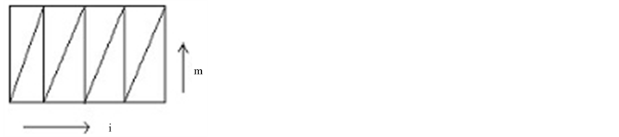
Figure 7. This is a  triangulation, the diagonals of each rectangle represents a regular fiber
 .
.
 (15)
(15)
and  is identified with
  the isometry group preserving orientation is
 . Hyperbolic planes are hemispheres and we have the concept of points at infinity. A fine feature of hyperbolic geometry is the fact that infinite objects can have finite volumes. This is the case of the ideal tetrahedron (one having one or more points at infinity). See [21] .
We now follow the Thurston geometrization conjecture [22] to construct our space.
We cut a manifold along essential spheres and tori. We take a connected component of the result of this process, completing spheres with balls and adding the “torus at infinity” in order to obtain the so-called “end” of the manifold. A graphical representation of this is the Figure 9.
Note: If we cut the cusp, we can visualize it as if we cut along a Euclidean plane in the upper half space model and see the previous movements associated to the toroidal boundary. This gives the eigenvalues . From the last statement we have the abelian group
 . This is the acting group in the
  manifold.
4.3.1. Cusp Hyperbolic Space
Here we construct our hyperbolic space with a single cusp and toroidal boundary.
Consider first the cube  which is composed as follows:
Gluing face  with
with  and
and  to
to  (following the direction of the arrows in the cube of the Figure 10), we obtain a cusp hyperbolic space and boundary homeomorphic to a 2-dimensional torus as we can see in Figure 11.
The above construction gives the definition of a cusp.
We need the two-dimensional torus, since in the next section we need to glue the boundary homeomorphically to a torus with either SF-sphere or SFH-sphere.
4.3.2. Cusp Hyperbolic Space Triangulation
We describe in this part a triangulation of a cusp hyperbolic space , from a triangulation on the torus.

Figure 11. Cusp hyperbolic space with toroidal boundary.
Based on [8] and [9] (with the same ideology) do the following:
Take a partition from a toroidal boundary, with the number of rectangles  (where
  are Seifert hyperbolic invariants).
The details are as follows:
We have first  and
and , i.e. we have two triangles, then we will generalize in order to obtain a formula for the number of generated tetrahedra.
Take the rectangle with vertices , in
, in . We denote by
  the points at infinity. Now we take the four points at infinity
  (we will call the resulting cube as
 ) and construct the following tetrahedra
 ;
; 


 and finally the tetrahedron formed by
 . Similarly, as in SFH-triangulation we have the number of generated tetrahedra in this case 6 (see Figure 12).
As we need to generalize this process for  and
and , we have, in this case, two glued cubes.
For the cube  (showed in Figure 13) we have then 12 tetrahedra, namely
 .
.
Note that by gluing  with
with  and
and  with
with  the tetrahedra of the partition does not generate new vertices, since the figures have symmetrical form. Not having new vertices the gluing will not generate any more tetrahedra.
Generalizing this process for any  and
and , we have:
That is, in Figure 14 we see that for each cube  we have 6 tetrahedra. If for example
  and
and  then we have 12 cubes, i.e.
  then we will have 72 tetrahedra. The following result is obtained by the above.
 (16)
(16)
With this we triangulated our cusp hyperbolic space obtaining also the number of generated tetrahedra, given by 
In Section 5 we will construct our model and we will use splice diagrams which are similar to graphs.
5. Model of a Universe with a Fundamental Interaction
In our topological model, each fundamental interaction is characterized by the following pair of parameters 
 . These will be related to an assembly
  of topological spaces composed of Seifert fibered spheres and a cusp hyperbolic space for each singular orbit. With the triangulations obtained in the preceding sections.
Each  interaction is related to an assembly
  of topological spaces
 , which are interpreted as a set of allowable 3-spatial sections of the “universe” with one fundamental interaction. See [6] and [27] .
We begin by describing the assemblies . See [10] for the discrete volume.
We take a Seifert fibered sphere (SF-sphere),  of the family
 (17)
(17)
which contains two regular and two singular orbits as described in the Subsection 4.2 and we associate the fol-

Figure 12. Note that each cube  has inside five mixed tetrahedra, i.e. each tetrahedron may have only 2 or 3 or even 1 point at infinity.

Figure 13. Where C has its vertices at infinity.
lowing splice diagram.

Notation: the second subscript denotes the level  for
for  we have
  and
and .
.
Removing the torus neighbourhoods of singular orbits and introducing the torus part of a cusp hyperbolic space by a splice operation (see [17] ). Then we have constructed a new manifold denoted by 
 (18)
(18)
and the corresponding splice diagram.

With this process we removed singular orbits and exchanged them by cusp hyperbolic spaces.
Now, consider a SF-sphere  containing two singular and two regular orbits (this is the zero level) and another SF-sphere
 , containing three singular and three regular orbits (this is level one).
In (18) we have glued two hyperbolic spaces, in order to glue in . The end of
  with
with ; but in
  we must first remove the hyperbolic space
  and then we will glue
  _ with
  applying a splice operation. After that, we add two hyperbolic spaces (also level one) in the singular orbits
  and
and  of level one SF-sphere. Here
For the construction of the assembly  we need to define the following manifold:

In other words, we are indicating that the splice operation was made in singular orbit  of
of  (which corresponds to
  invariant), and
  (corresponding to
  invariant) as well as
  and
and  invariants. We remove one toroidal neighbourhood at each singular orbit and it is replaced by the corresponding
  space. For this we associate the splice diagram below.

Then the assembly will be defined by:
 (19)
(19)
The  components are obtained from
  manifold using the connected sum
  times between
  sub manifold. Where
  is the tubular neighbourhood of a singular orbit
  extracted from SFsphere
  using a splice operation. We remove singular orbits of
  and replaced them by a cusp hyperbolic spaces.
Generalizing this idea we get.

Finally, all singular orbits are removed and replaced by either another SFH-sphere or by a cusp hyperbolic space, fulfilling our goal of avoiding singular orbits (no singular points). See [10] for the discrete volume of this new manifold and a comparison with coupled constants.
6. Conclusions
In our construction we remove the tubular neighbourhoods of singular orbits and replace them by a hyperbolic space thus achieving two things. First, avoiding singularities from any space is closer to a physical representation. Usually it is hard to have a physical representation when in theory we have a singularity. Instead, we can imagine singular points as points at infinity. Second, we construct a different space than Efremov and Mitskievich did, introducing Thurston’s theory and using the work done by Knesser, Milnor, Jaco, Shalen, Johanson. This space shows an improvement for the calculation of the hierarchy of the coupling constants, i.e. reproducing more closely the exponents of the coupling constants. This is important because the use of hyperbolic spaces instead the local use of hyperbolic geometry make a better approach.
Building the model of the universe with 3-dimensional spatial sections from Seifert fibered homology spheres and cusp hyperbolic spaces provides a description of the evolution at least for the hierarchical approach of the coupling constants by means of topological changes. We also use manifolds which contain a finite volume. Therefore, we can calculate volumes in these spaces. In other words, we have an infinite space with finite volume.
We have created here a new cusp hyperbolic space with fibers. This allows calculating the volume of this particular manifold. Once we obtain how to calculate the volume of each tetrahedra in the space, only what we need is to multiply for the number of tetrahedra contained in the cusp hyperbolic space. All of this is due to the space which was discretized. And this could be used in cosmology theories for calculating the volume density of the space.
As a final comment, we emphasize the importance of the approach presented here for the study of alternative cosmological models. Highlighting an important example, the standard Friedmann Singularity-Free (FSF) theories usually consider more complex structures than the simple spherically symmetric point like a Friedmann singularity (the big bang seed with null dimension and infinite density). Following this path, we point out here a possible application of the topological construction introduced in this paper to cosmological scenarios known as “Cusp Cosmology” which are based on the cusp-like geometries resulting from non-linear wave theory [29] .
Acknowledgements
Thanks to: Ignacio Barradas, Klaus-Peter Schröder, César Caretta, Hugo Garca, Stephanie Dunbar and Lawrence Nash. CONACyT, LAC-INPE, CAPES and PROAP.
Appendix
Orbifold
Here we take the definition given by [21] .
Definition 8. An orbifold  is a space locally modelled on
  modulus finite group actions.
  consists of a Hausdorff space
 , with some additional structure.
  has a covering that consists of a collection of open sets
  closed under finite intersections. To each
  is associated a finite group
 , an action of
  on an open subset
  of
of  and a homeomorphism
 . Whenever
 , there is an injective homomorphism

and an embedding

equivariant with respect to  (i.e. for
 ) such that the next diagram commutes.

Next we describe some helpful orbifold characteristics.
Definition 9. A point  in a 2-dimensional orbifold
  is a cone point with a cone angle
 , if there exists a neighbourhood around
  which is an orbifold diffeomorphic to the quotient orbifold
 , where
  is the group of the p-roots of the unit.
Notation: We will denoted by  a closed orientable Seifert manifold which admits a fibration with basis, where
  is the Seifert fibration.
Note that the pair , (where
  for
for ) are given by the exceptional fiber. We consider
 ,
,  are not necessarily relative primes. The last two are given by the exceptional fibers (singular). The genus
  characterizes the base space, which is the connected sum of
  torus if
  We have the 2-sphere when
  and the connected sum of
  projective planes when
  The rational Euler class
  represents an obstruction to the existence of a section of the fibration, since by reversing the orientation of
 , reverses also the orientation of the fibers or the base (it does not matter which because
  admits an orientation preserving the automorphic mapping of fibers in fibers). We replace the Seifert invariant
  by
by  then
then  If
If , changing some
  to
to , then we have
  Henceforth, we will assume that
  when
when  denoting such manifold by
Like homology spheres are a particular case of SFM, here is the follow definition.
Definition 10. Homology spheres. Let  be co prime integers with
  and each
  Then there is a 3-SFM, with a Seifert invariant that has the form

with
 (20)
(20)
This manifold is denoted by  and it is a homology sphere.
By  we denote that
  is not there.
For any oriented Seifert fibered homology sphere . There is a unique n-tuple
  with single orientation sign
 , such that
  This orientation preserves homeomorphisms. This homeomorphism can be chosen to preserve the Seifert fiber structure. As an additional reference on fiber bundles we refer reader to might look [30] .
Topological Description of Homology Spheres
Let  be a n-fold of the 2-punctured sphere, then
  can be characterized by an oriented closed 3-manifold in which we can immerse pairwise disjoint solid torus
  such that:
1) If 
then, exists a fibration  with fiber
  so
so 
2) If  is a section of
  and for

then  is null homologous to
  where each
  satisfies (20).
We remark that (0.20) determines  and
and . In a geometric description we have that
  y
y  depend on the choice that we make of the section
  See [17] .
NOTES
1The fibers play the role of a coordinate basis for objects in the field.