Optical Spectrometer with Acousto-Optical Dynamic Grating for Guillermo Haro Astrophysical Observatory ()
1. Introduction: General Characterization of the Spectrometer
The Cassegrain telescope, which is in operation at the Guillermo Haro astrophysical observatory (Mexico), includes classical static grating spectrometer (from Boller & Chivens Corp.). Presently, this spectrometer is available on the observatory at the 2.12-meter telescope with 5 static diffraction gratings, see Table 1. All the static gratings are 9 cm × 9 cm in size, and they are exploited in the first order of light diffraction with the dispersions ranging from 450 to 114 , allowing a good coverage in both dispersion and wavelength within the CCD matrix photodetector sensitivity ranges. The use of acousto-optics techniques in astronomy starts from the late 1960s when a new kind of spectral devices was developed, electronically tunable acousto-optical filters (AOFs). Later, in the middle of the 1970s [1], the first efforts to use the tunable AOFs for astronomical spectroscopic observations were made at the Harvard Observatory in 1976. Using a collinear filter is based on calcium molybdate crystal. Conceptually and technologically,

Table 1. Static diffraction gratings available in the Guillermo Haro astrophysical observatory.
AOFs at that time were imperfect. The filter had a small optical aperture (4 × 4 mm) and a large interaction length . Now, the tunable AOFs are technologically mature, compact tunable AOF-based spectrometers and cameras are widely used for research and process control. For example, acousto-optics is widely used currently for spectroscopy in radio-astronomy. In 2002, imaging spectrophotometer on optical range with CCD cameras was tested [2]. More examples exist for the use of acoustooptics in astrophysical spectroscopy, such as SPICAM in Mars Express [3].
As usually, the converging light beam from the telescope passes through the spectrometer entrance slit in the telescope focal plane to the collimator, an off-axis parabolic mirror. The reflected parallel beam then falls on to the diffraction grating surface. The diffracted light passes through a Schmidt camera, which images the spectrum on to the CCD matrix. This optical spectrometer can be characterized by the following parameters.
1.1. Efficiency of the Static Diffraction Grating
The efficiency as well as the dispersion at the desired working wavelength is an important parameter when choosing a diffraction grating. The efficiencies of the available static gratings have been measured experimentally, so that one of them, exhibiting the maximum diffraction efficiency up to 70%, is presented in Figure 1 as an example. It should be noted that the total system efficiency is the combination of the efficiencies of the telescope, spectrometer, grating, camera, and the detector, but diffraction efficiency of the dispersive element plays the key role.
1.2. Spectral Coverage
The static grating dispersion, camera focal length, and detector size determine the joint observable spectral range. For example, a grating with the slit-density 300 lines/mm with a blaze angle , which has a dispersion of
  when grating is used in the first order of diffraction, will provide a spectral coverage of
 , where M is the number of pixels on the dispersion axis in the detector. With a detector of 1024 pixels,
 .
.

Figure 1. Maximum diffraction (reflection) efficiency of the static diffraction grating with: the slit-density 300 lines/mm, dispersion 224 , and blaze angle of
 : solid line is for the light polarized parallel to slits and dashed line is for the light polarized perpendicular to slits [4].
1.3. Spectral Resolution
The theoretical spectral resolution depends on the static grating dispersion, grating position, pixel size, collimator and camera focal lengths, and entrance slit-width. The effective CCD matrix spectral resolution also depends on the detector sampling. As an example, static grating with 300 lines/mm and with the blaze angle  will have theoretical resolutions of 2.24 and 4.48 Å for slit-widths of 1" and 2", respectively. Decreasing the entrance slitwidth will improve the spectral resolution. However, this will be possible only when the sampling requirements (Nyquist criterion; one resolution element imaged onto at least two detector elements) are respected and also when the instrumental response is not diffraction limited. Within exploiting a CCD matrix, the effective spectral resolution is determined by convolution between the spectrograph resolution
  of pixels per a resolvable spot and the detector pixel size. With suitable pixel sizes, the spectrum may be sufficiently sampled to avoid spectral information distortion (e.g. instrumental broadening). The most common sampling criterion is
  (i.e. Nyquist criterion). Due to the current needs of astrophysical observations the resolution of spectrometer has to be changed time to time that can be done only by mechanical substitution of one static diffraction grating with another one. Every time the static grating is substituted, the spectrometer needs to be realigned and recalibrated; however, it leads to potential errors in measurements and losing very important physically and rather expensive time for the observations.
In order to improve this situation, we propose an alternative for the static diffraction gratings, namely, to use specially designed acousto-optical cell as the dynamic diffraction grating, which is electronically tunable and whose capabilities will make it possible in the nearest future to replace the static diffraction gratings from the spectrometer with the new acousto-optical cell. The principal advantages of similar dynamic acousto-optical grating are excluding any mechanical operations within the observation process, avoiding recalibrations (i.e. bringing in additional errors) and any losses of time. Potentially, applying the acousto-optical technique, which can realize tuning of both the spectral resolution and the range of observation electronically, makes possible eliminating these demerits. Additionally, one can expect increasing the efficiency of the spectrometer’s operation, because a dynamic diffraction grating in the form of specially designed acousto-optical cell is able potentially to provide close to 100% efficiency of spectrum analysis.
2. The Nature of Acousto-Optical Dynamic Diffraction Grating
The photo-elastic effect consists in connection between the mechanical deformations  or stresses
  and the optical refraction index
 . This effect takes place for all the condensed matters and mathematically can be explained as [5]
 , (1)
, (1)
where  represents varying the tensor of optical impermeability or, what is the same, the parameters for an ellipsoid of optical refractive indices; while
  is the tensor of photo-elastic coefficients. Usually, the higher-order terms relative to the deformations
  are omitted due to smallness about
  of even linear deformations
 . The symmetry inherent in a medium determines non-zero factors of the tensor
 . With nonzero external mechanical perturbations, an ellipsoid for the refractive indices can be explained by
 . (2)
. (2)
Now, let us consider propagation of the traveling single-frequency longitudinal elastic wave along the acoustic axes noted as  -axes. The main property of each acoustic axis in anisotropic acousto-optical material is its ability to support just pure acoustic modes, longitudinal or/and shear ones, within their propagation through. This property is almost the same what can be met in isotropic materials. This is why for simplicity sake one may consider the longitudinal acoustic mode passing through an isotropic medium with scalar refractive index n which can be the average one in a crystal. So that pure longitudinal displacement
  of particles is described by
 , where
  and
and  are the amplitude, cyclic frequency, and wave number of that elastic wave, respectively. The field of linear deformations
 , occurred by this wave, is
 . The components of the optical impermeability tensor can be written as a)
 b)
b) , (3)
, (3)
while  for the indices
 . Due to the tensors
  and
and  are symmetrical in behavior, one can use so-called matrix indices, so that here
  are the components of the photo-elastic tensor
  with the above-mentioned matrix indices
  [5].
[5].
In this case, Equation (2) gives
 . (4)
. (4)
Due to Equation (4) does not include any cross-terms, the main axes inherent in a new ellipsoid for the refractive indices will have the same directions as before. Consequently, new main values  of the refractive indices can explained as a)
 b)
b) . (5)
. (5)
These equations mean that in the presence of the traveling acoustic wave, the taken isotropic medium becomes a periodic structure, which is equivalent to a bulk grating with the grating constant equal to the acoustic wavelength , because variations in the main refractive indices
  and
and  are proportional to the amplitudes of displacement or/and deformations in that acoustic wave. An example for a sinusoidal variation of the refractive index is illustrated in Figure 2. This periodic perturbation in a medium is varying in space and in time as well. It represents a traveling wave propagating with the ultrasound velocity
 , whose magnitude in the condensed matters is typically equal to about
 . However, the light velocity exceeds this magnitude by about 5 orders, so that periodic perturbations conditioned by that acoustic wave can be always considered as quasi-static in behavior relative to light propagation. Thus, potential resolution R of similar diffraction grating measured in the number of slits per unit aperture D (let us say, for
 ) or, what is the same, the stroke density can be determined by the ratio
 .
.
3. Novel Schematic Arrangement
A new configuration of the spectrometer under proposal, which has already included the dynamic acousto-optical grating as a dispersive element instead of traditional static diffraction grating, is shown in Figure 3.
The light coming from the telescope will pass through a slit: solid lines represent the light beam, being coaxial to the collimator normal, while both dotted and dashed
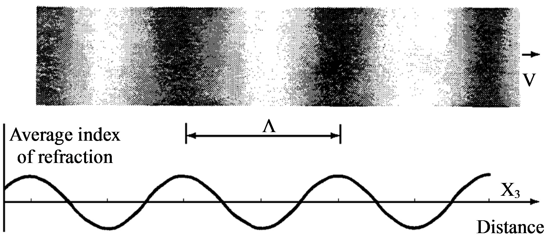
Figure 2. The instantly frozen acoustic wave, which consists of alternating with one another areas of compressed and decompressed material density and the corresponding sinusoidal variations of the average refractive index.

Figure 3. Schematic arrangement of the acousto-optical version of optical spectrometer: black lines represent the light beam, being coaxial to the collimator normal, while blue and red lines represent light beams slightly tilted from that normal.
lines represent light beams slightly tilted from that normal. The slit is placed on the focal plane of the collimating mirror. The aperture of the slit will limit the angular range of the observation. The collimated beam will arrive to the acousto-optical cell at the Bragg angle, for the previously selected wavelength, and then it will be diffracted. Then, the diffracted light will be imagined in the CCD matrix by a lens or, to have the less possible losses, by a Schmidt camera.
The practical aspects of designing an updated version of the schematic arrangement for spectrometer under consideration lead first of all to creation of a modified optical scheme, which has to include some peculiarities of the AOC. Figure 3 represents the modified configuretion of the spectrometer using the AOC as dynamic diffraction grating instead of the static diffraction gratings; here,  is the Bragg angle of light incidence for the chosen optical wavelength, see below Equation (9). The light coming from the telescope will pass through the spectrometer entrance slit at the focal plane of the collimator mirror, the reflected beam, a plane wave, will fall on to the AOC at the Bragg angle. Then, the diffracted beams corresponding to the first order will be imaged using a Schmidt-camera and analyzed. An additional modification is connected with the fact that the acoustooptical dynamic diffraction grating operates sufficiently effective in the Bragg transit regime instead of the reflection regime inherent in the above-mentioned classical spectrometer whose static diffraction gratings exhibit about 70% maximum efficiency.
4. Estimating the Acousto-Optical Materials
The requirements to the acousto-optical cell (AOC) combine a large optical aperture with the needed slit-density R, an acceptable level of uniformity for acoustical grooves limited by linear acoustical losses in the chosen material, and possibly high efficiency of operation under an acceptable applied acoustic power. The list of the, currently in use, static diffraction gratings was shown in Table 1. This is why initially we have restricted ourselves by the given slit-density (for example, R = 300 lines/mm), which leads to the inequality 
 , where
 , i.e. to the requirement
 . (6)
. (6)
The other requirement is connected with the uniformity of acoustical grooves is restricted by the acoustic attenuation, whose level B along the total optical aperture D of AOC should not exceed a given value, which can be determined as 6 dB due to usual requirements related to the dynamic range of analysis. The acoustic attenuation is usually almost square-law function of the carrier acoustic frequency f [6]. Let us use the conventional factor  of acoustic attenuation [7] expressed in
 . Thus various forms of limitations connected with acoustic attenuation can be written. For example, the total level
  of acoustic attenuation can be expressed as
 . (7)
. (7)
Table 2 demonstrates the carrier frequencies f allowing us to realize the AOC, which provide the slit-density R = 300 lines/mm together with the potential total losses along the AOC aperture.
Then, a given value of  for the acoustic attenuation will require the aperture of
  or the carrier frequency
 (8)
(8)
at a given optical aperture D within the chosen acoustooptical material. It is naturally to search for the materials allowing the choice of the carrier acoustic frequency  satisfying the combined inequality
 . Selecting appropriate materials is conditioned by low enough acoustical losses per aperture and after that as high as possible figure of acousto-optical merit
 . Considering those values, one can find that a few crystalline materials exhibit attractively low level (i.e. close to
 ) of acoustical losses, wherein only two of them, namely,
  and
and  manifest relatively larger figure of acousto-optical merit
 . Thus, one can formulate that in the case of R = 300 lines/mm,
  , and
, and , which leads to the following choice:
1)
 ,
,  ,
,
 :
:  and
and

Table 2. Estimations for the carrier frequencies f and the corresponding total acoustic losses  along the AOC with a 9 cm-aperture for the dynamic grating with the slit-density of R = 300 lines/mm. Values of the factor
 , acoustic velocity V, and figure of acousto-optical merit M2 are borrowed from Ref. [8,9].
 ;
;
2)
 ,
,  ,
,
 :
:  and
and
 .
.
Here,  and
and  are the slow shear acoustic mode and the longitudinal one, respectively. They both are pureacoustic modes, providing exact coincidence between the wave vectors and the energy flow vectors with the chosen directions (in fact, with the acoustic axes in crystals) of these elastic waves propagation.
The Bragg regime of light diffraction occurs with a large enough length L of acousto-optical interaction. In this case the dynamic acoustic grating is rather thick, so that during the analysis of diffraction one has to take account of the phase relations between light waves in different orders. When the incident light beam is unlimited in a transverse direction, the reflected beam will be placed in the plane of incidence (i.e. in the  -plane) and the angle of reflection should be equal to the angle
  of incidence. The coupled-mode theory predicts that a considerable reflection of the incident light can be expected under condition
 , (9)
, (9)
where  is the light wavelengths, while
  is the whole number, which reflects the
  Fourier component of the perturbed dielectric permeability. In the case of pure sinusoidal profile peculiar to the acoustic wave, all the Fourier-components with
  will be equal to zero. Thus, the Bragg regime can be realized only when the angle of light incidence
  on a thick dynamic acoustic grating meets the Bragg condition
  and inequality
  for the Klein-Cook parameter [10]. Usually, when an acoustic mode is exited by the applied electric signal, the Bragg regime includes the incident and just one scattered light modes, whose normalized intensities under condition of zero mismatches are described by [11]
a) b)
b) c)
c) d)
d) , (10)
where  is the space coordinate almost along the light propagation;
  is the acoustic power density,
  is the material density,
  is the effective photo-elastic constants for light scattering, and n is now the averaged effective refractive index of a material. The Bragg regime is preferable for practical applications due to an opportunity to realize a 100% efficiency of light scattering by the acoustic wave. Taking the case of
  in Equation (10b) and
  in Equation (10c), one can find from these equations that the acoustic power density
  needed for 100% efficiency of light diffraction into the first order can be estimated through the requirement
  in Equation (10b) as
 . (11)
Thus, at the same values of optical wavelength  and the interaction length
 , the required acoustic power density will be inversely proportional to the acousto-optic figure of merit
 . For the above-mentioned orientations of crystals, one can say that [8,9]:
(1)  (
(
 ,
, )
) ;
;
(2)  (
( ,
,  ,
, )
) .
.
For reaching 100% efficiency of operation at, for example,  and
and , the following acoustic power densities
  can be found from Equation
(11): (1)  (
(
 ,
, )
)
 ;
;
(2)  (
( ,
,  ,
, )
)
 .
.
Here,  and
and  are the slow shear acoustic mode and longitudinal one, respectively, passing along the corresponding axes. They both are pure acoustic modes, providing exact coincidence between the wave vectors and the energy flow vectors with the chosen directions (in fact, with the acoustic axes in crystals) of these elastic waves propagation. At this step, it should be explained additionally: applying the needed electronic signals at the electronic input of AOC in such a way that the aboveobtained levels of acoustic power density will be provided makes it possible physically and potentially technically to achieve 100% efficiency of control over the incident light diffraction. By the other words, instead of about 70% maximum efficiency shown in Figure 2 for traditional static diffraction gratings, involving the acousto-optical technique via creating the dynamic acoustooptical diffraction gratings is potentially able to provide close to 100% efficiency of dispersive element over all the range of the above-mentioned spectrum analysis. This fact is caused by an active nature of AOC, which manifests some quantum gain controlled by an external variable electronic signal, in the contrast with traditional static acoustic grating.
Then, in the particular case of , one can estimate the resolution of the AOC as a dispersive element. The above-mentioned Bragg condition can be rewritten as
  and differentiated with respect to the acoustic frequency
 , so that one can obtain
 . Because the frequency resolution peculiar to an AOC in the optical scheme with space integrating is given by
 , one can find that
 . (12)
Consequently, in the above-chosen case of R = 300 lines/mm,  , and
, and , one can estimate
 , which is valid for both the selected materials:
(1)
 ,
,  ,
,
 ,
, ;
;
(2)
 ,
,  ,
,
 ,
, .
.
One can see from Equation (12) that potential spectral resolution of the AOC as dispersive element is high enough in comparison with the data presented in Table 1. Thus the dynamic acousto-optical grating can be considered as rather perspective component for the optical spectrometer under discussion.
5. Diffraction of the Light Beam of Finite Width by a Harmonic Acoustic Wave at Low Acousto-Optic Efficiency
Schematic arrangement of the acousto-optical version of spectrometer, see Figure 4, exhibits potential presence of optical beams whose widths are restricted due to condition of observations. This is why the diffraction of light beam of finite width by harmonic acoustic wave has to be reviewed and characterized. At first, to illustrate the existing physical tendency simpler let us start from a low acousto-optical efficiency approximation
 , where now
  is the angular-frequency mismatch. Due to almost orthogonal geometry of non-collinear acousto-optical interaction the angles of incidence
  and diffraction
  do not exceed usually about 10˚, so that one can use the simplified formulas a)
 b)
b) c)
c) , (13)
where  is the average refractive index;
  are the refractive indices for the incident or diffracted light, respectively.
Now, we assume that the area of propagation for a harmonic acoustic wave is bounded by two planes  and
and  in a crystal. This acoustic wave has the amplitude function
  with the amplitude
 , wave number
 , and cyclic frequency
 , and travels along
  -axis. Then, let initially monochromatic light beam incidents on the area of interaction under the angle
 . At the plane
 , the light field is described by the complex valued amplitude function
 , reflecting the spatial structure of light field. The spectra of these fields are [12]
a) b)
b) , (14)
where  is the wave number of the incident light. Each

Figure 4. Geometry of interaction between light and acoustic beams.
individual component of the incident light beam is diffracted by the acoustic harmonic in the interaction area. Using Equations (13) and (14) within taken low acoustooptical efficiency, the angular spectrum of the diffracted light can be written as [13]
 , (15)
 .(16)
.(16)
Equation (15) describes AOC as linear optical system with the transmission function , which is realvalued (and positive) within its bandwidth, i.e. AOC does not insert phase perturbations in the spectrum of optical signal.
When the width  of the incident light beam is less than acoustic aperture of AOC, one can say that acoustic beam is infinitely wide, while light beam is described by the complex amplitude function
 , where
  only when
  and
and
 when
when . Its angular Fourier spectrum is given by
 . (17)
Substituting Equation (17) in Equation (15), one can obtain angular distribution for the diffracted light intensity at low acousto-optical efficiency.
a) b)
b) c)
c) . (18)
The functions  and
and  represent angular spectra of light and acoustic beams. The diffracted light structure is determined by overlapping the functions
  and
and , i.e. by relation between the light divergence angle
  and the acoustic one
 , so that the Gordon parameter
  had been introduced [14]. With
 , the widths of
  and
and  have the same order. When
 , one can simplify Equation (18a) as
 ; with

 , one yields
 . These peculiarities of diffracting light beam of finite width are illustrated by Figure 4. The diffracted light waves take their origin in all the points of overlapping light and acoustic beams. Due to their interference, these waves shape the diffracted light beam, propagating at the angle
 . The diffracted light width
  can be estimated by
 .
.
This relation can be rewritten as , where
 . Thus the divergence angle of the diffracted light is close (in its order of quantity) to the smallest divergence angle of the interacting beams.
The acousto-optic efficiency  can be determined as ratio of the diffracted light intensity to the incident light intensity when both
  and
and  from Equations (17) and (18a) will be integrated over the corresponding angle ranges:
 . (19)
Efficiency of diffraction for the plane incident light wave has maximum efficiency at , and the term
 , describing the acousto-optical efficiency for plane incident light wave, is marked out here to highlight the contribution of light beam finiteness. However, Bragg condition cannot be provided now for all the angular components described by Equation (17). This is why one can chose the angle of incidence
  in such a way that the phase synchronism condition will be satisfied for the axis-component of incident beam. In the case of
  with
with , one can obtain [15], see Figure 5.
 (20)
(20)
Equation (19) should be compared with the above taken relative intensity of diffraction  for
for

Figure 5. The factor  versus the Gordon parameter
 .
.
plane optical waves at low acousto-optical efficiency. One can see from Equation (19) that a finite width of the incident light beam leads to appearing an additional factor  depending only on the Gordon parameter
 . The factor
  reaches unity only in the limit of
 , which corresponds to the case of plane incident light wave. Growing the Gordon parameter makes acousto-optical interaction worse. Physically, this effect is motivated by the fact that exact phase synchronism can be realized only for one, namely, axis-component of light beam, while all other components are diffracted with lower efficiency.
Within Bragg diffraction of a high acousto-optical efficiency, the factor , conditioned by acoustic power density
  via Equation (10c), has to be taken into account. The transmission function
  from Equation (16) should be substituted by
 ,(21)
,(21)
This modification leads ultimately to another expression for efficiency , which is similar to Equation (19). As before, the term
 , describing the diffraction of high efficiency for plane incident light wave, is marked out to exhibit the contribution of light beam finiteness, while the function
  reflects the same tendency as
 . Anyway, finally one can conclude that when AOC operates over the light beams of finite width, decreasing the acousto-optical efficiency due to partial asynchronism for the divergent incident light beam cannot be eliminated.
6. Conclusions
We have suggested exploiting an acousto-optical cell (AOC) as a dispersive element in optical spectrometer of the Guillermo Haro astrophysical observatory (Mexico). Potentially, involving acousto-optical technique, which can realize tuning both the spectral resolution and the range of observation electronically, makes possible eliminating the above-mentioned practical demerits and excluding filters. The requirements to the cell combine a large optical aperture with the needed slit-density and possibly high efficiency of operation under an acceptable acoustic power. This is why initially we have restricted ourselves by the slit-density 300 lines/mm along the 9 cm aperture. The analysis has shown that at least the following materials can be used for designing similar AOC. It can be lithium niobate  -crystal excited by the longitudinal acoustic mode along the [100]-axis at the frequency 2 GHz. This selection gives 300 lines/mm with total losses ~5.3 dB/aperture. Then, one can consider bismuth germanate
  -crystal using the shear acoustic mode along the [110]-axis at 0.53 GHz, so that the slit-density 300 lines/mm appears with the losses ~6.3 dB/aperture. The neighboring figures of acoustooptical merit for these materials promise desirable efficiencies of operation, so that even close to 100% efficiency peculiar to the dynamic acousto-optical dispersive element over all the range of the spectrum analysis can be expected. The figures of acousto-optical merit
  for these materials are neighboring and promise efficiencies of operation sufficient for observations.
The proposed schematic arrangement for the acoustooptical version of optical spectrometer is able to reduce dimensions and weight of a system in a view of operating over the spectral range of wavelengths 400 - 800 nm. Potential performances of an AOC as the dynamic diffraction grating look rather attractive for practical applications due to their potential spectral resolution as dispersive element is about δλ ≈ 0.184Å, which looks rather attractive in comparison with the data presented in Table 1. Finally, diffracting the light beam of finite width by a harmonic acoustic wave at low acousto-optic efficiency has been briefly discussed.
7. Acknowledgements
This work has been financially supported by the CONACyT (Mexico), project # 151494.