Training a Quantum Neural Network to Solve the Contextual Multi-Armed Bandit Problem

Wei Hu¹, James Hu²

¹Department of Computer Science, Houghton College, Houghton, NY, USA.
²Department of Computer and Information Science, University of Pennsylvania, Philadelphia, PA, USA.

DOI: 10.4236/ns.2019.111003                

Abstract

Artificial intelligence has permeated all aspects of our lives today. However, to make AI behave like real AI, the critical bottleneck lies in the speed of computing. Quantum computers employ the peculiar and unique properties of quantum states such as superposition, entanglement, and interference to process information in ways that classical computers cannot. As a new paradigm of computation, quantum computers are capable of performing tasks intractable for classical processors, thus providing a quantum leap in AI research and making the development of real AI a possibility. In this regard, quantum machine learning not only enhances the classical machine learning approach but more importantly it provides an avenue to explore new machine learning models that have no classical counterparts. The qubit-based quantum computers cannot naturally represent the continuous variables commonly used in machine learning, since the measurement outputs of qubit-based circuits are generally discrete. Therefore, a continuous-variable (CV) quantum architecture based on a photonic quantum computing model is selected for our study. In this work, we employ machine learning and optimization to create photonic quantum circuits that can solve the contextual multi-armed bandit problem, a problem in the domain of reinforcement learning, which demonstrates that quantum reinforcement learning algorithms can be learned by a quantum device.

Keywords

Continuous-Variable Quantum Computers, Quantum Machine Learning, Quantum Reinforcement Learning, Contextual Multi-Armed Bandit Problem

1. Introduction

In recent years, the research and application of artificial intelligence has experienced a revolution and has sparked an explosion of interest, fueled by its astonishing performance, supported by more powerful computing, more efficient algorithms, and more data. Machine learning as a part of AI is an area in computer science that studies the question of teaching computer models how to learn from data. Among the three major categories of machine learning: supervised, unsupervised, and reinforcement learning, reinforcement learning is closest to what people tend to think of artificial intelligence. When a learning agent is placed in an unknown environment, supervised learning would teach the agent the correct actions to take, while in a reinforcement learning setting, only the rewards for these actions are provided to the agent, which are weaker signals than those in supervised learning. Supervised and unsupervised learning can be considered as learning about the data, but reinforcement learning is learning to behave or how to take actions (Figure 1). The goal of reinforcement learning is for the agent to maximize the total cumulative reward by learning a good strategy from the environment and the rewards it received [1 - 3].

The advances in mathematics, materials science, and computer science have made quantum computing a reality today. Making use of the counterintuitive and distinctive properties of superposition, entanglement, and interference of quantum states, quantum computing is a new computing paradigm based on the laws of quantum mechanics. Quantum computers can process information more efficiently than traditional computers and provide us with a platform to enhance classical machine learning algorithms and to develop new quantum learning algorithms [4 - 15].

The qubit-based quantum computer can represent discrete variables naturally, but cannot represent continuous variables efficiently. The continuous-variable (CV) quantum computing architecture [16] can use the measurements of common quantum observables such as position or momentum to represent continuous variables naturally, with an infinite-dimensional bosonic mode as the basic information-processing unit in this model. The CV models allow information to be encoded and processed much more compactly and efficiently than qubit-based models, which fit well with the actual needs of machine learning, in particular, deep learning that uses continuous vectors and tensors as their fundamental computational units.

Deep learning has impressed people with its AI abilities demonstrated by numerous applications such as AlphaGo from Google. The mathematical structure of deep learning is supported by a multi-layered neural network where the output of one layer is used as an input to the next. Each layer is made of a number of neurons where a linear transformation of the input is conducted, followed by a nonlinear activation function. Mathematically, these neural networks can approximate any continuous functions, which are commonly used in machine learning.

The quest for quantum neural networks has been a long journal. One of the challenges is the design of the nonlinear activation function in each layer of the network while maintaining the unitary property of the operation. In the CV quantum architecture, this problem is solved seamlessly, by using non-Gaussian gates to provide both the nonlinearity and the universality of computation. Quantum neural networks offer a quantum advantage, where in some problems, a classical neural network would require an exponential number of resources to approximate a quantum network. To fully take advantage of the quantum and classical computing, a hybrid quantum-classical technique to create quantum circuits with a variational approach has been proposed [17]. This versatile method uses a quantum device to evaluate the cost function of a model, a computationally intensive task, and uses a classical device to optimize the model.

Figure 1. A typical reinforcement learning diagram: after an agent takes an action when in a certain state, it will receive a reward and move to a next state.

Quantum machine learning can improve classical machine learning. One well-known classical learning technique is kernel methods, which maps lower dimensional data into higher dimensional space, sometimes infinite-dimensional, but requires lengthy computational time when the dimension is high. Recent works show that quantum devices can do this kind of calculation naturally and efficiently. In a continuous-variable photonic quantum system, a classical data point can be prepared as an input quantum state to a quantum circuit. This quantum state is a vector in an infinite dimensional Fock state, so it is already in an infinite dimensional space without the help of the kernel trick [18].

2. Related Work

The goal of quantum machine learning is to use quantum processors to develop novel quantum algorithms that can dramatically accelerate computational tasks for machine learning. The recent development of hybrid quantum-classical technique fits well with the current state of quantum technologies.

The work in [19] takes a variational approach to design photonic quantum circuits in the continuous-variable (CV) architecture to process information stored in quantum states of light, in which the quantum gates have free continuous parameters to fine tune. The circuits are made of photonic quantum gates: interferometers (phase shifters and beam splitters), squeezing and displacement gates, and nonlinear gates. These photonic circuits can form a sequence of repeating building blocks, or layers, with the output of one layer serving as the input to the next. This structure of layers is similar to those in the classical neural networks. The functionality of this quantum networks is also similar to that of their classical counterparts. The interferometers and squeezing gates match the weight matrix in the classical network, the displacement gates act as the bias, and the quantum nonlinearity serves as the classical nonlinear activation function. A subsequent work [20] is using machine learning to optimize a quantum neural network circuit to produce arbitrary quantum states. Once the correct parameters are learned, this state-preparation subroutine can then be reused within other quantum circuits or algorithms. In this instance, classical machine learning is helping to train a quantum neural network.

Using a combination of Gaussian and non-Gaussian gates, these circuits provide the nonlinearity necessary to create quantum natural networks, unitarity of quantum operations, and universality of computation. They magically maintain highly nonlinear transformations while keeping operations completely unitary. Our work designs a circuit of photonic quantum computers to solve the contextual multi-armed bandit problem [21 - 24] using machine learning and optimization techniques. This circuit is made of optical gates with free continuous parameters optimized by the photonic quantum computer simulator Strawberry Fields [25].

3. Methods

Our study employs a reinforcement learning technique, a policy gradient, to train the quantum neural network. So we introduce the policy gradient first.

3.1. Policy Gradient for Reinforcement Learning

The aim of reinforcement learning is to train a learning agent to discover a good strategy in order to receive the maximum cumulative rewards through interaction with the unknown environment. In the domain of reinforcement learning, the strategy is usually termed as a policy that maps states to actions, either deterministically or stochasticatically. There are two major approaches to learning a good policy: value-based and policy-based methods. The former learns state values V(s) and action-state values Q(s, a) and then based on these functions, find a good policy $\pi \left(a|s\right)$ . The latter directly learns a good policy $\pi \left(a|s\right)$ , which is the method we use in this study. Although we could define a policy $\pi \left(s\right)=\arg {\max }_{a}Q\left(s,a\right)$ if Q(s, a) is found, in general we may have little interest in knowing the exact value of Q(s, a). Another reason for us to find the policy directly is when the action space is continuous or the environment is stochastics, computing Q(s, a) becomes a complicated task.

To explain our work, we only introduce the policy gradient algorithm in the episodic environment. First we introduce a parameter $\theta$ to the policy function $\pi \left(a|s\right)={\pi }_{\theta }\left(a|s\right)=P\left[a|s,\theta \right]$ then use the gradient of this policy to find a $\theta$ that can produce maximum cumulative rewards. Running one episode, the whole trajectory of the agent is recorded as $h=\left\{s_1,a_1,r_1,s_2,a_2,r_2,\cdots ,s_T,a_T,r_T\right\}$ . The policy objective function $J\left(\theta \right)$ is defined as $J\left(\theta \right)={\displaystyle \int {\pi }_{\theta }\left(h\right)r\left(h\right)\text{d}h}$ where r(h) is a reward function. Using a common trick of ${\pi }_{\theta }{\nabla }_{\theta }\log {\pi }_{\theta }={\nabla }_{\theta }{\pi }_{\theta }$ , the policy gradient algorithm REINFORCE [26] can be stated as the following:

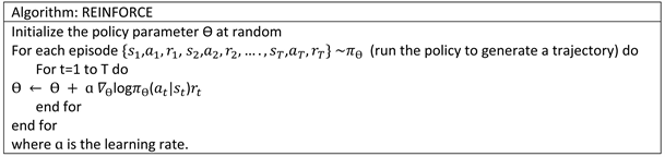
In the original multi-armed bandit problem, the state remains fixed as there is only one bandit while in the contextual multi-armed bandit problem, the state changes as there are several bandits. The updating rule of REINFORCE encourages actions that receive positive rewards while penalizing those that do not. In general, policy gradient methods work better than the value based such as Q learning since the policy gradient directly optimizes the reward but the training can be a challenge because of the high variance of rewards that makes the algorithm unstable.

3.2. Photonic Quantum Circuits for Machine Learning

Different from the more commonly known qubit-based models, continuous-variable quantum computing is a universal computing model which can process continuous variables. In a CV model, information is stored in the quantum states of bosonic modes, called qumodes and the CV quantum circuits are unitary in the Hilbert space picture, but they can have nonlinear effects in the phase space picture when non-Gaussian gates are used, a fact that is critical for designing CV quantum neural networks.

Inside a CV quantum circuit the quantum gates usually contain free parameters which allow for a variational approach to optimize them for a particular machine learning task (Figure 2). Quantum gates are tools to control how quantum states evolve through unitary operations. Mathematically these gates can be represented as unitary matrices with complex-valued entries. A real-valued vector $X=\left(x_1,x_2,\cdots ,x_N\right)$ in N-dimensional space is represented as N-mode quantum optical states $|X\rangle =|x_1\rangle \otimes |x_2\rangle \otimes \cdots \otimes |x_N\rangle$ . In this report, our numerical analysis is conducted with Strawberry Fields [25] which is a quantum simulator for photonic circuit design. Strawberry Fields has advanced functionality and applications for quantum computing and quantum machine learning.

To introduce the photonic gates, we denote the creation operator by $a^{†}$ and annihilation operator by a. The displacement gate is $D\left(a\right)=\exp \left(a{a}^{†}-a^{\ast }a\right)$ and squeeze, rotation, and Kerr single mode gates are defined as $S\left(r\right)=\exp \left[\frac{r}{2}\left(a^2-a^{†}{}^2\right)\right]$ , $R\left(\varphi \right)=\text{exp}\left(i\varphi \hat{n}\right)$ , and $K\left(\kappa \right)=\text{exp}\left(i\kappa {\hat{n}}^2\right)$ respectively, where $\hat{n}=a^{†}a$ is the number operator. The two mode bean-splitter is $BS\left(\theta ,\varphi \right)=\exp \left[\theta \left({\text{e}}^{i\varphi }{a}_1^{†}{a}_2-{\text{e}}^{-i\varphi }{a}_1{a}_2^{†}\right)\right]$

which creates entanglement between the two modes. The visual representation of the effects of some of these gates is shown in Figure 3. The quantum circuit in Figure 4 consists of the successive gate sequences that represent unitary transformation on 4 qumodes. Gaussian gates are single or two-mode gates which are at most quadratic in the mode operators, while non-Gaussian gates are single-mode gates which are degree 3 or higher.

Figure 2. Variational quantum circuit: the quantum gates in the circuit collectively define a unitary operation on quantum states and these gates depend on classical parameters ϴ. The output of the circuit is classical and therefore it is a good candidate for optimizing it by updating the values of ϴ according to a specific learning objective using classical machine leaning and optimization techniques. In our study, we apply the policy gradient to tune ϴ.

Figure 3. Wigner function representation of vacuum state, squeezed vacuum state, rotated vacuum state, Kerr state (applying Kerr gate to a coherent state), displaced vacuum state, displayed in sequence.

Figure 4. The actual circuit structure for a CV quantum neural network used in this study: interferometer, displacement, rotation, squeeze, and Kerr (non-Gaussian) gates. The detailed definition of these gates can be found in [25].

In this work, we use four qumodes to construct a quantum neural network. The input to the circuit represents the action in the multi-armed bandit problem, and also the state in the contextual multi-armed bandit problem. The output of the circuit is the photon number measurements that represent the four weights on the four arms in the bandit. The goal of the policy gradient training of the circuit is to output the weights that guide the agent to choose the right arm to gain the maximum reward. Our network has a total of 32 gates from a universal set for CV quantum computing. Compared to the multi-layered quantum neural networks in [19], our circuit can be considered as a single layer network, which is sufficient to solve the current problem. When several different models can all solve the same problem, the simplest model is preferred.

Due to the use of non-Gaussian gates, this circuit can produce nonlinear transformation while maintaining its unitary property as a whole. The non-Gaussian gates are also necessary ingredients to build a universal quantum computing model. The Kerr gate is used because it is diagonal in the Fock basis, which leads to faster and more reliable numerical simulations when compared with the cubic phase gate, another well-known non-Gaussian gate.

3.3. Contextual Multi-Armed Bandit Problem

The multi-armed bandit problem can be described using this analogy. Say there is one slot machine with multiple arms. Each arm has an unknown but fixed probability of giving out a prize. We can try one arm at a time, and our aim is to find a strategy to maximize our cumulative rewards. In this environment, there is just one state, one slot machine, and only the action can vary. The description of contextual bandits requires the concept of the state, which can serve as an extra clue that the agent can use to take more informed actions. In the contextual multi-armed bandit problem, there are N slot machines with multiple arms, which is an extension of the previous problem. In this case the state, the slot machine, can vary as well. Now the goal of the agent is to learn the best action not just for a single bandit, but for any number of them. Contextual bandits can be used to optimize random allocation in clinical trials and enhance the user experience for websites by helping choose which content to display to the user, ranking advertisements, and much more.

To balance the trade-off between exploitation and exploration, we employ the ε-greedy algorithm which means with a small probability ϵ the agent takes a random action, but otherwise it picks the best action according to the output of the quantum neural network. There is already a significant amount of attention given to supervised and unsupervised learning research, but relatively less progress has been made for reinforcement learning [6 , 7]. The main goal of our study is demonstrate that quantum neural networks can be used to solve problems in reinforcement learning, adding a quantum solution to the rich collections of classical methods such as ε-greedy, upper confidence bounds (UCB), and Thompson sampling [22 - 24].

A multi-armed bandit is a tuple (A, R) where A is a known set of actions or arms and R(r|a) = P(r|a) is an unknown probability distribution over rewards. At each step t, the agent selects an action $a_t\in A$ and the environment generates a reward $r_t\in R\left(.|a_t\right)$ . The goal of the agent is to find a good strategy in

obtaining the maximum cumulative reward ${\displaystyle {\sum }_{t=1}^{t=T}{r}_t}$ . The contextual multi-armed bandit problem can be

defined similarly as a tuple (S, A, R) where S is a collection of states [21 - 24].

4. Results

In this work, we have conducted two experiments. One is to train a quantum neural network, a learning agent in this study, to solve the multi-armed bandit problem, and the other is to solve the contextual multi-armed bandit problem where the extra dimension is having states in the problem. The training method is ϵ greedy, which means ϵ% of the times, actions are selected at random while the rest of the times the quantum neural network is used to select the actions. In this study, we chose ϵ = 0.1. Each bandit has four arms with each arm having a different but fixed probability to produce a positive reward 1 or a negative reward −1. In the contextual multi-armed bandit problem there are four bandits, and consequently this problem has four states.

4.1. Multi-Armed Bandit Problem

In this problem, there is only one bandit, which has four arms in this study. We select two arms of the bandit to have higher probability to give a positive reward than the other two in the first experiment. Then we switch the two highest probabilities to see if the quantum neural network is able to detect the change in the second experiment. The experiments of training the quantum neural network for 500 steps show that it can identify the two arms of the top two positive rewards in each case (Figure 5). The payout probabilities for each arm in each experiment are listed in Table 1.

4.2. Contextual Multi-Armed Bandit Problem

In this problem, there are four bandits, with each having four arms in this study. We select one arm of each bandit to have the highest probability of generating a positive reward than the other three (Table 2). Then we try to see if the quantum neural network can identify the arm of the best payout in each bandit. The experiments of training the quantum neural network for 1000 steps show that it can discover the arm of the best payout in each bandit (Figure 6).

Table 1. The payout probabilities for each arm in the two experiments for bandit problem.

Figure 5. The learning curves for the agent to detect the arm of the highest probability of getting a positive reward.

Figure 6. The learning curves for the agent to detect the arm of the highest probability of obtaining a positive reward in each bandit.

Table 2. The payout probabilities for the four arms in each bandit in the experiments for contextual bandit problem.

5. Conclusion

Quantum computers make use of the properties of quantum physics to process information much faster than their classical counterparts. As a result, quantum technologies provide a fertile ground to explore new ideas and models in computation that could potentially revolutionize the ways of how information is stored and processed. The real benefit of using quantum computing is to efficiently solve certain problems that are extremely expensive for classical computers. Driven by new algorithms, increased computing power, and big data, deep learning structured by multi-layer neural networks has demonstrated its great power in many different areas, thus, bringing in great interest in learning how to create quantum neural networks. Quantum variational algorithms are recently proposed as a hybrid between classical and quantum computing, in which a classical computer varies certain free parameters to control the preparation of quantum states, and then a quantum computer prepares the states.

The quantum analogue of the classical bit is the qubit which can represent discrete variables naturally, but cannot represent continuous variables efficiently. However in machine learning, continuous variables are commonly used so continuous-variable quantum systems are more suitable in the design of quantum neural networks. In a classical neural network, the nonlinear activation function plays an important role in approximating any continuous functions. However, in quantum physics, the operations on quantum states are required to be linear and unitary, a restriction that brings great difficulty when creating quantum neural networks. In a photonic quantum system, this nonlinearity is achieved by the non-Gaussian gates. We need to understand what advantages may arise from generating the superposition, entanglement, and interference of quantum states during operations of the quantum neural networks.

In this report, we showcase the application of variational methods to create photonic quantum neural networks that can solve the contextual multi-armed bandit problem, where the agent is trained with a policy gradient to gain maximum cumulative rewards. Compared to some other problems in reinforcement learning where the rewards are delayed, the rewards in the contextual multi-armed bandit problem are immediate. Our work also highlights that classical machine learning can aid quantum computers in learning in the domain of reinforcement learning, allowing quantum and classical learning to complement each other.

Conflicts of Interest

The authors declare no conflicts of interest regarding the publication of this paper.

References

[1]	Sutton, R.S. and Barto, A.G. (2018) Reinforcement Learning: An Introduction. 2nd Edition, A Bradford Book.
[2]	Ganger, M., Duryea, E. and Hu, W. (2016) Double Sarsa and Double Expected Sarsa with Shallow and Deep Learning. Journal of Data Analysis and Information Processing, 4, 159-176. https://doi.org/10.4236/jdaip.2016.44014
[3]	Duryea, E., Ganger, M. and Hu, W. (2016) Exploring Deep Reinforcement Learning with Multi Q-Learning. Intelligent Control and Automation, 7, 129-144. https://doi.org/10.4236/ica.2016.74012
[4]	Farhi, E. and Neven, H. (2018) Classification with Quantum Neural Networks on Near Term Processors. arXiv:1802.06002.
[5]	Dong, D.Y., Chen, C.L., Li, H.X. and Tarn, T.-J. (2008) Quantum Reinforcement Learning. IEEE Transactions on Systems, Man, and Cybernetics, Part B (Cybernetics), 38, 1207-1220. https://doi.org/10.1109/TSMCB.2008.925743
[6]	Biamonte, J., Wittek, P., Pancotti, N., Rebentrost, P., Wiebe, N. and Lloyd, S. (2017) Quantum Machine Learning. Nature, 549, 195-202. https://doi.org/10.1038/nature23474
[7]	Dunjko, V. and Briegel, H.J. (2018) Machine Learning and Artificial Intelligence in the Quantum Domain: A Review of Recent Progress. Reports on Progress in Physics, 81, 074001. https://doi.org/10.1088/1361-6633/aab406
[8]	Hu, W. (2018) Empirical Analysis of a Quantum Classifier Implemented on IBM’s 5Q Quantum Computer. Journal of Quantum Information Science, 8, 1-11. https://doi.org/10.4236/jqis.2018.81001
[9]	Hu, W. (2018) Empirical Analysis of Decision Making of an AI Agent on IBM’s 5Q Quantum Computer. Natural Science, 10, 45-58. https://doi.org/10.4236/ns.2018.101004
[10]	Hu, W. (2018) Towards a Real Quantum Neuron. Natural Science, 10, 99-109. https://doi.org/10.4236/ns.2018.103011
[11]	Hu, W. (2018) Comparison of Two Quantum Clustering Algorithms. Natural Science, 10, 87-98. https://doi.org/10.4236/ns.2018.103010
[12]	Ganger, M. and Hu, W. (2019) Quantum Multiple Q-Learning. International Journal of Intelligence Science, 9, 1-22. https://doi.org/10.4236/ijis.2019.91001
[13]	Naruse, M., Berthel, M., Drezet, A., Huant, S., Aono, M., Hori, H. and Kim, S.-J. (2015) Single-Photon Decision Maker. Scientific Reports, 5, Article ID: 13253. https://doi.org/10.1038/srep13253
[14]	Naruse, M., Chauvet, N., Jegouso, D., Boulanger, B., Saigo, H., Okamura, K., Hori, H., Drezet, A., Huant, S. and Bachelier, G. (2018) Entangled Photons for Competitive Multi-Armed Bandit Problem: Achievement of Maximum Social Reward, Equality, and Deception Prevention. arXiv:1804.04316.
[15]	Mitarai, K., Negoro, M., Kitagawa, M. and Fujii, K. (2018) Quantum Circuit Learning. arXiv:1803.00745.
[16]	Serafini, A. (2017) Quantum Continuous Variables: A Primer of Theoretical Methods. CRC Press, Boca Raton. https://doi.org/10.1201/9781315118727
[17]	Peruzzo, A., McClean, J., Shadbolt, P., Yung, M.-H., Zhou, X.-Q., Love, P.J., Aspuru-Guzik, A. and O’Brien, J.L. (2014) A Variational Eigenvalue Solver on a Photonic Quantum Processor. Nature Communications, 5, Article No. 4213. https://doi.org/10.1038/ncomms5213
[18]	Schuld, M. and Killoran, N. (2018) Quantum Machine Learning in Feature Hilbert Spaces. arXiv:1803.07128
[19]	Killoran, N., Bromley, T.R., Arrazola, J.M., Schuld, M., Quesada, N. and Lloyd, S. (2018) Continuous-Variable Quantum Neural Networks. arXiv:1806.06871
[20]	Arrazola, J.M., Bromley, T.R., Izaac, J., Myers, C.R., Brádler, K. and Killoran, N. (2018) Machine Learning Method for State Preparation and Gate Synthesis on Photonic Quantum Computers. arXiv:1807.10781
[21]	http://www0.cs.ucl.ac.uk/staff/d.silver/web/Teaching_files/XX.pdf
[22]	Auer, P., Cesa-Bianchi, N. and Fischer, P. (2002) Finite-Time Analysis of the Multiarmed Bandit Problem. Machine Learning, 47, 235-256. https://doi.org/10.1023/A:1013689704352
[23]	Collier, M. and Llorens, H.U. (2018) Deep Contextual Multi-Armed Bandits. arXiv:1807.09809
[24]	Tekin, C. and Turgay, E. (2018) Multi-Objective Contextual Multi-Armed Bandit with a Dominant Objective. arXiv:1708.05655
[25]	Killoran, N., Izaac, J., Quesada, N., Bergholm, V., Amy, M. and Weedbrook, C. (2018) Strawberry Fields: A Software Platform for Photonic Quantum Computing. arXiv:1804.03159
[26]	Williams, R.J. (1992) Simple Statistical Gradient-Following Algorithms for Connectionist Reinforcement Learning. Machine Learning, 8, 229-256. https://doi.org/10.1007/978-1-4615-3618-5_2