The Macroeconomic Impact of Shocks in the US Federal Funds Rate on the Republic of South Africa: An SVAR Analysis

Moeti Damane

Central Bank of Lesotho, Maseru, Lesotho.

DOI: 10.4236/me.2018.94053                

Abstract

This study empirically examines the influence of shocks in the US federal funds rate on the Republic of South Africa’s output gap, consumer prices, 91-day T Bill rate and the Rand-US Dollar exchange rate from the first quarter of 1981 to the last quarter of 2014 with the use of a structural vector autoregressive (SVAR) model. Shocks in the US federal funds rate are found to have more of an impact on the South African inflation rate relative to other domestic macro variables. Domestic developments were found to play the most significant role in explaining the fluctuations of South Africa’s macro-variables. In light of the SARB’s inflation targeting monetary policy regime, it is recommended that it remains mindful of domestic developments as well as movements in the US federal funds rate in order to determine their upside risks to inflation before deciding on a policy stance.

Keywords

US Federal Funds Rate, South Africa, SVAR, Impulse Response, Variance Decomposition

1. Introduction

The ever increasing pace of globalisation has resulted in a profound level of interconnectedness among the world’s countries. This development has led to economies being vulnerable to external shocks¹ that translate into enhanced volatility across domestic macroeconomic variables [1] together with [2] . The notion that greater integration between the world’s economies and financial systems has deepened over the years is hardly refutable. Reference [3] pointed out that economic discussion around the interdependence of national economies is nothing new and has occupied economic thinking from as far back as the 1960s and 1970s when models of open economies such as those developed by Robert Mundell and Marcus Fleming interrogated the effects of shocks in one economy on its trading partners. Reference [4] [5] [6] [7] along with [8] noted the importance of evaluating how globally integrated monetary policy and monetary policy shocks, especially those from the developed world are transmitted internationally to the least developed and developing worlds. They advanced that a key advantage in this endeavour is that investors and policy makers from the developing world are provided with a clear understanding of the implications of monetary policy decisions from developed countries, especially on capital flows between the developed and developing world. Reference [4] [9] and [10] posited that empirical investigations into the impact of monetary policy from large economies on other economies more often than not focuses on the role of the United States (US) in international transmission of monetary shocks with the key focus being changes in the US federal funds rate. Interestingly, in the case of the Republic of South Africa (South Africa), [11] noted that the US is one of the country’s top five export trading partners and was the second most important destination for its exports in 2015 after China. It is against this backdrop that this paper investigates the impact of a shock in the US policy rate (the federal funds rate) on a set of macroeconomic variables from South Africa, a country with a floating exchange and an inflation targeting monetary policy regime.

Over the years, there have been a number of studies dedicated to assessing the influence of shocks in US monetary policy on other economies. These include [6] [7] [9] [10] [12] and [13] . While these studies undeniably provide insightful information into the impact of US monetary policy shocks on other countries; they seldom focus on the effect of shocks in US monetary policy on developing countries from the sub-Saharan African (SSA) region, or South Africa in particular. Moreover, the impact of external monetary policy shocks on domestic economies depends on the specific set of macro-variables included in various research models. Reference [14] noted that currently, a standard list of variables for inclusion into macroeconomic monetary policy analysis does not exist. Reference [15] underscored that selection of variables can be formal or informal. The choice of macro variables in this research paper does not follow any formal selection process but is guided by the work of [8] [13] [16] as well as [17] . The aim of this paper is two-fold. First, to evaluate the response of South African macroeconomic variables, specifically, consumer prices, output gap, 91-day Treasury bill rate and the Rand-US Dollar exchange rate to a shock in the US federal funds rate by using quarterly time series data spanning the first quarter of 1981 to the last quarter of 2014. Second, determine the importance of US monetary policy shocks in explaining changes to South African macroeconomic variables. The rest of the paper is organised as follows: Section 2 provides a brief background of the South African Reserve Bank’s (SARB’s) monetary policy framework since the 1980s with specific interest on the current inflation targeting monetary policy regime. Section 3 reviews the relevant literature. Section 4 presents materials and methods. Section 5 outlines the empirical results. Section 6 details the robustness checks. Section 7 concludes the study.

2. Brief Background of the South African Reserve Bank Monetary Policy Framework since the 1980s

Reference [18] together with [19] noted that in the 1980s, SARB’s monetary policy implementation strategy was chiefly concerned with maintaining a stable financial environment. This was seen as a crucial precondition towards the containment of inflation, the promotion of high and sustainable economic growth, increased levels of employment and the overall improvement in the living standards of the country’s residents. As pointed out by [18] coupled with [20] , SARB monetary policy in the 1980s was based on monetary targeting. Monetary policy decisions were undertaken with due cognisance of the changes in the growth rate of domestic broad money (M3) supply. Overtime, greater global financial market integration, the liberalisation of the South African capital market and the relaxation of exchange controls made the conduct of monetary policy much more challenging than it was during the time of Apartheid², when South Africa was broadly isolated from external shocks. The challenge manifested itself in longer time lags between policy changes and the desired impact on the real economy and inflation. This rendered monetary targeting an undesirable monetary policy strategy [18] .

With the ever increasing inadequacy of monetary targeting in informing credible monetary policy decisions SARB had to shift to a monetary policy strategy that was more in tune with the dynamics of the world South Africa found itself in. Reference [21] highlighted that in the 1990s, SARB’s monetary policy framework eventually moved away from monetary targeting and adopted what is known as the eclectic approach to monetary policy decision making. Under this approach, a handful of indicators³ were studied and their movements determined the SARB’s monetary policy stance. The ultimate intention was for SARB to move towards an explicit inflation targeting regime as this framework was widely adopted across the world by various central banks [18] . According to [19] [20] as well as [22] , the SARB formally adopted an inflation targeting framework on 6 April 2000. The adoption of an explicit inflation targeting framework signalled that SARB would no longer solely rely on monetary aggregates (the growth in money supply and bank credit extension) to guide determination of short-term interest rates. Reference [19] explained that under an explicit inflation targeting regime the SARB would have to undertake a detailed assessment of a number of domestic⁴ and foreign⁵ indicators when deciding on an appropriate monetary policy stance. Reference [20] and [23] discussed that the SARB’s inflation target aims at achieving a rate of increase in headline consumer price index⁶ (CPI) of between 3 and 6 per cent per year. Reference [22] pointed out that the repo rate⁷, which is the rate that the SARB charges commercial banks for borrowed cash reserves, is the main instrument used to target inflation. Figure 1 presents SARB’s monetary policy transmission mechanism (MPTM) under the inflation targeting framework. It articulates the process through which the SARB achieves its monetary policy goals.

From Figure 1, the SARB’s monetary policy transmission channels are nominal exchange rate, commercial bank rates, asset prices (bond, equity and real estate prices) as well as expectations. The ultimate target is the inflation rate. Consider a contractionary monetary policy stance (a rise in the repo rate) whose aim

Source: South African Reserve Bank.

Figure 1. SARB monetary policy transmission mechanism.

would be to quell the rise in inflation. First, a rise in the repo rate will affect the nominal exchange rate by causing an appreciation in the SA domestic currency, the rand. The country’s imports become cheaper relative to exports and these result in a deterioration of the trade balance that ultimately shrinks the aggregate demand. A slowdown in demand translates into a reduction in the level of production, wages, employment and ultimately prices of goods. Second, in response to the hike in the repo rate, commercial banks respond by raising their loan prices (bank lending effect). This is likely to adversely affect private sector demand for credit, consumer confidence and investment. Not only that, the increase in bank lending rates implies an increased cost of servicing existing debt, which generally erodes the disposable income of economic agents. On the contrary, returns on savings and investment increase in reaction to higher interest rates but consumers could cut back on savings in light of the higher cost of servicing debt. Third, increases in the repo rate affect asset prices negatively as the market value of bonds, equities and real estate decreases. This reduction in asset values compromises wealth from investments and decreases spending. Last, the repo rate changes affect expectations of economic agents regarding future developments in economic variables which in turn can have an impact on aggregate demand and inflation.

3. Literature Review

3.1. Theoretical Literature

3.1.1. The Traditional Mundell-Fleming-Dornbusch (MFD) Model

Reference [1] and [24] explained the Mundell-Fleming-Dornbusch (MFD) model as an open economy version of the IS-LM in which capital movements, monetary variables and exchange rates form an integral part of its design. Furthermore, the MFD was developed to analyse macroeconomic policy in a small open economy under the assumption that such an economy is a price taker in the import and export markets. Reference [13] acknowledged that the single country MFD and later its two-country version are widely considered to have led the way in international macroeconomic modelling. Reference [1] and [9] explained that under a floating exchange rate regime and perfectly mobile capital, the intrinsic results of the two-country MFD given an expansionary monetary policy depict a “beggar-thy-neighbour” policy framework such that the domestic economy (where the expansionary policy is enacted) benefits while the foreign country suffers. Specifically:

1) After a monetary expansion, the nominal interest rate falls in the expanding country;

2) This leads to a capital outflow, which then leads to a depreciation of the currency of the expanding country;

3) This will mean the other country has experienced a currency appreciation;

4) The currency depreciation in the expanding country is incentive for an increase in exports, a reduction in imports and a subsequent improvement in the trade balance;

5) The currency appreciation in the other country means a decrease in exports and an increase in imports and a resultant deterioration in the trade balance;

6) The improved trade balance and depressed interest rate in the expanding country translate into a rise in its output;

7) The output in the other country experiences a fall due to the deterioration in its trade balance with the expanding country.

According to [9] , under perfect capital mobility and a fixed exchange rate regime, the MFD posits that contractionary monetary policy leads to monetary contraction in the domestic and foreign countries. However, when flexible exchange rate regimes and imperfect capital mobility are considered, a contraction in monetary policy in the domestic country results in a reduction of its price level and output coupled with an increase in consumer prices in the foreign countries as a result of exchange rate changes. When the Mundell-Fleming trilemma or impossible trinity is considered, [25] noted that an economy that chooses to fix the value of its currency and have independent monetary policy cannot have freely flowing capital across its borders. Furthermore, if the economy has a fixed exchange rate and free flowing capital across its border, it cannot have an independent monetary policy. Last, if the choice is to have free flowing capital across borders and monetary autonomy, it is not possible to operate under a fixed exchange rate regime. According to [26] , what then becomes important is the effectiveness of domestic monetary policy under the trilemma, especially in the face of changes in the monetary policy stance of a relatively bigger economy like the US. In such circumstances, the Mundellian idea of a policy mix where monetary policy and fiscal policy are used complementarily to arrive at the desired effect could find favour [27] .

3.1.2. The Intertemporal Model

Reference [28] and [29] explained that intertemporal models of the current account gained prominence in the 1980s when researchers sort to understand the implications of modelling the current account by taking into consideration the assumptions of forward looking economic agents whose forecasts of relevant variables hinged on rational expectations. Reference [30] pointed out that [28] bridged the gap in open economy model building by developing a series of extended models that incorporated relative prices, complex demographic structures, consumer durables, asset-market incompleteness, and asymmetric information. Spurred on by the Lucas critique of economic policy evaluation, the intertemporal approach was therefore developed to replace the MFD model.

Reference [28] presented an open economy version of the sticky price closed economy model by expanding it to a two country open model and adding a foreign asset accumulation component together with assumptions around the exchange rate, interest rates, capital markets and capital mobility. Under this intertemporal model, economic agents (households and firms) must determine their optimal levels of:

・ Aggregate consumption dynamics (and thus asset holdings);

・ Relative demand for different goods (composition of aggregate demand); and

・ Production effort for own good.

According to [30] , analysis in the intertemporal model covers three periods; the initial steady state (time t − 1), the period when the shock hits (time t), and the period after the shock, when the economy adjusts to the new steady state (time t + 1). Moreover, the main transmission channel of a shock in the short run is the nominal exchange rate while the transmission of a shock in the long run is through wealth redistribution between countries. Reference [27] and [30] noted that the intertemporal model conforms to the basic predictions of the MFD model in the initial stages of a monetary shock. That is, given a positive shock in monetary policy in a foreign country, this will lead to a fall in interest rates in the domestic economy and domestic economy currency depreciation coupled with a temporary increase in domestic income. However, due to consumption smoothing by economic agents, the level of domestic consumption rises by a magnitude less than that of domestic income. This means an improvement in the domestic economy’s current account.

3.2. Empirical Literature

Reference [31] evaluated the role of external factors in capital inflows and exchange rate appreciation in ten Latin American countries using a structural vector autoregression (SVAR) model and monthly data from January 1988 to December 1991. The study used variance decompositions to assess the relative importance of external shocks in explaining forecast error variations in reserves and real exchange rates. Results concluded that for countries that did not experience any major shifts in domestic policy over the sample period, for example; implementation of stabilisation plans and adoption of floating exchange rates, external shocks accounted for a significant shift (about 50 per cent) in the monthly forecast error variation in real exchange rate and reserves. However, there were puzzles. Foreign factors were found to account for the least variation in the forecast error of exchange rates and reserves in countries that had significant changes in their domestic policy during the period under consideration. In addition, results of the impulse response functions indicated that for a handful of the countries under consideration, a positive shock to US monetary policy (a contractionary monetary policy) led to a currency appreciation and an increase in reserves in the foreign country.

Reference [4] used an SVAR model and annual time series data covering the period January 1986 to December 2000 to ascertain the extent to which macro-variable fluctuations in emerging markets in Asia and Latin America were attributable to international shocks. In the paper, external factors are divided into “US monetary policy” and “everything else” or “private sector shocks”. This decomposition proved crucial since it revealed that less than 10 per cent (in most cases) of the variation in domestic macro-variables could be tied to shifts in US monetary policy, implying that private sector structural shocks were more important. This discovery is similar to that of [31] .

Reference [12] analysed the international monetary transmission mechanism of US monetary policy shocks in non US G-6 countries under a flexible exchange rate period using a vector autoregression (VAR) methodology. The study concluded that expansionary shocks in US monetary policy translate in positive effects in non US G-6 countries. Moreover, the US trade balance is found to worsen in the short-term after the expansionary shock although it improves in the medium and long term. The findings are therefore not in support of the postulations of the basic version of the MFD model.

Reference [6] studied the impact of shocks in US monetary policy on eight Latin American countries with the use of a VAR model and quarterly time series data from the first quarter of 1990 to the second quarter of 2002. The impact of shocks in US monetary policy are investigated on five macro-variables measuring real activity, inflation, interest rates, trade and international competitiveness. The study concluded that the interest rate channel is the most important transmission mechanism of US monetary shocks to Latin America while the trade channel plays a negligible role. The author identified three possible reasons for this. First, the majority of debt in these countries is denominated in US Dollars; therefore, financial markets may force the increase in Latin American interest rates following an increase in the default risk from such countries. Second, in an attempt to stem capital outflow, Latin American central banks adjust rates upwards. Third, given the sheer size and importance of the US economy in the global space, a contractionary monetary policy in the US leads to a general increase in world interest rates. The overall result is therefore an increase in capital flows to Latin American countries, an improvement in central bank reserves together with an increase in aggregate demand and consumer prices.

Reference [9] examined the changing international transmission of US monetary policy shocks to fourteen OECD countries over the first quarter of 1981 and the last quarter of 2010 with the help of a factor augmented VAR and a time-varying parameter factor VAR. The study found that contractionary shocks in US monetary policy result in a negative impact on the output growth in the US, Canada, Japan and Sweden while exhibiting positive effects on the output growth in most of the other OECD member countries. The asset prices, interest rates, and the trade channel were identified as the most significant drivers in the transmission of monetary policy shocks from the US to the OECD countries.

Reference [7] investigated the impact of monetary policy shocks emanating from the Euro Area (EU) and the US on a group of eleven sub-Saharan African (SSA) countries. The countries included those following a fixed exchange rate regime and those with a floating exchange rate regime like South Africa. Using an SVAR methodology, the results of the study were found to depend on whether the shock in monetary policy emanated from the EU or the US. Moreover, the results depended on whether the SSA country under consideration operated under a floating or fixed exchange rate regime. SSA countries with a floating exchange rate were found to have negative output response after a contractionary shock to either EU or US monetary policy. It was discovered that SSA countries that heavily relied on international capital increased their interest rates following a contractionary monetary shock from either the EU or US in order to stop capital from flowing out. This result is similar to the one observed under [6] . However, in the SSA case, the process led to depressed output growth. Reference [7] also noted that SSA countries operating under a fixed exchange rate regime depicted mixed output responses in the earlier periods but showed expansionary effects in the medium and long term. For these countries, the interest rate and trade channels acted as transmission mechanisms. US shocks were found to not be significant in SSA countries operating under a fixed exchange rate regime. Be that as it may, output in such SSA countries continued to expand, implying that some other factor, such as aid from the US was responsible for curbing the output contractions.

4. Materials and Methods

4.1. Materials

The study uses quarterly time series data from the first quarter of 1981 to the last quarter of 2014. From Table 1, the South African variables include the Rand-US Dollar exchange rate (ZARx), which is the price of one US Dollar (USD) in South African Rand terms, the 91-day treasury bill rate (R), the consumer price index (SAp) and the output gap (Ygap⁸). The US variable chosen is the federal funds rate (FedR). All of the data was obtained from the FRED database maintained by the US Federal Reserve Bank of St. Louis. The variables in the model are expressed in logarithmic form except R and FedR which are expressed in percentages.

South Africa’s 91 day T Bill rate is taken to proxy monetary policy innovations in the country since the SARB Repo rate data starts from 2001. In addition, [17] argue that innovations in the US federal funds rate are better indicators of monetary policy shocks than innovations in monetary aggregates. It is for this reason that the US Federal Funds rate is used as an indicator of monetary policy

Table 1. Variable description.

shocks in the US. Basing our a priori expectations on the postulations of the MFD model, it is expected that a positive shock to US monetary policy will lead to a decline in South African interest rates, a depreciation of the South African Rand against the US Dollar, an increase in South African output and an increase in the level of South African inflation.

4.2. Model Specification

The study estimates a VAR model to assess the response of South African output gap (Ygap), consumer prices (SAp), 91-day Treasury bill rate (R) and Rand-US Dollar exchange rate (ZARx) to shocks in the US federal funds rate (FedR). Reference [5] [32] and [33] posited that one of the most ideal tools for macroeconomic analysis is the VAR model pioneered by Christopher Sims in 1980. The VAR is arguably superior in its ability to navigate through dynamic effects of shocks to monetary policy on such macroeconomic variables as inflation, output and the exchange rate. They are also well suited for purposes of presenting the degree of influence of monetary policy shocks on developments in key macroeconomic variables.

The reduced form of the VAR is represented in Equation (1):

$X_t=G_0+G_1{X}_{t-1}+G_2{X}_{t-2}+\cdots +G_s{X}_{t-s}+{\epsilon }_t$ (1)

where $X_t$ is a (5 × 1) vector of endogenous macroeconomic variables (FedR, Ygap, SAp, R and ZARx) observed at time t. $G_0$ is a vector of constants, $G_{1,2,\cdots ,s}$ is a (5 × 5) matrix of coefficient estimates, ε is a (5 × 1) vector of serially uncorrelated system innovations and s is the optimal lag length of each variable. When unpacked, Equation (1) is a system of five equations as follows:

$\begin{array}{c}Fed{R}_t={\beta }_{1,0}+{\displaystyle {\sum }_{i=1}^s{\theta }_{1,i}Fed{R}_{i,t-1}}+{\displaystyle {\sum }_{i=1}^s{\lambda }_{1,i}Yga{p}_{i,t-1}}+{\displaystyle {\sum }_{i=1}^s{\varphi }_{1,i}SA{p}_{i,t-1}}\\ +{\displaystyle {\sum }_{i=1}^s{\varpi }_{1,i}{R}_{i,t-1}}+{\displaystyle {\sum }_{i=1}^s{\delta }_{1,i}ZAR{x}_{i,t-1}}+{\epsilon }_{1,t}\end{array}$ (2)

$\begin{array}{c}Yga{p}_t={\beta }_{2,0}+{\displaystyle {\sum }_{i=1}^s{\theta }_{2,i}Fed{R}_{i,t-1}}+{\displaystyle {\sum }_{i=1}^s{\lambda }_{2,i}Yga{p}_{i,t-1}}+{\displaystyle {\sum }_{i=1}^s{\varphi }_{2,i}SA{p}_{i,t-1}}\\ +{\displaystyle {\sum }_{i=1}^s{\varpi }_{2,i}{R}_{i,t-1}}+{\displaystyle {\sum }_{i=1}^s{\delta }_{2,i}ZAR{x}_{i,t-1}}+{\epsilon }_{2,t}\end{array}$ (3)

$\begin{array}{c}SA{p}_t={\beta }_{3,0}+{\displaystyle {\sum }_{i=1}^s{\theta }_{3,i}Fed{R}_{i,t-1}}+{\displaystyle {\sum }_{i=1}^s{\lambda }_{3,i}Yga{p}_{i,t-1}}+{\displaystyle {\sum }_{i=1}^s{\varphi }_{3,i}SA{p}_{i,t-1}}\\ +{\displaystyle {\sum }_{i=1}^s{\varpi }_{3,i}{R}_{i,t-1}}+{\displaystyle {\sum }_{i=1}^s{\delta }_{3,i}ZAR{x}_{i,t-1}}+{\epsilon }_{3,t}\end{array}$ (4)

$\begin{array}{c}{R}_t={\beta }_{4,0}+{\displaystyle {\sum }_{i=1}^s{\theta }_{4,i}Fed{R}_{i,t-1}}+{\displaystyle {\sum }_{i=1}^s{\lambda }_{4,i}Yga{p}_{i,t-1}}+{\displaystyle {\sum }_{i=1}^s{\varphi }_{4,i}SA{p}_{i,t-1}}\\ +{\displaystyle {\sum }_{i=1}^s{\varpi }_{4,i}{R}_{i,t-1}}+{\displaystyle {\sum }_{i=1}^s{\delta }_{4,i}ZAR{x}_{i,t-1}}+{\epsilon }_{4,t}\end{array}$ (5)

$\begin{array}{c}ZAR{x}_t={\beta }_{5,0}+{\displaystyle {\sum }_{i=1}^s{\theta }_{5,i}Fed{R}_{i,t-1}}+{\displaystyle {\sum }_{i=1}^s{\lambda }_{5,i}Yga{p}_{i,t-1}}+{\displaystyle {\sum }_{i=1}^s{\varphi }_{5,i}SA{p}_{i,t-1}}\\ +{\displaystyle {\sum }_{i=1}^s{\varpi }_{5,i}{R}_{i,t-1}}+{\displaystyle {\sum }_{i=1}^s{\delta }_{5,i}ZAR{x}_{i,t-1}}+{\epsilon }_{5,t}\end{array}$ (6)

Equation (1) can be estimated using the ordinary least squares (OLS) method. The choice of optimal lag order will be made with due consideration of information criterion such as the Schwarz Information Criterion (SIC) and or Akaike Information Criterion (AIC). The smallest information criterion between is the most preferred. Once the appropriate lag order has been selected, the stationarity of the system, or the stability of the system is tested with the help of the AR roots table. The system will be found to be stationary if the modulus of each root is within the unit circle.

4.3. Unit Root Tests

Reference [33] explained that VAR models are designed for stationary variables. To ascertain the order of integration of the variables, the study uses Augmented Dickey and Fuller (ADF) test as explained in [34] and [35] as well as the Phillips-Perron (PP) test as explained in [36] . The PP test complements the ADF in that it is non-parametric and corrects for any serial correlation and heteroskedasticity in the errors. The two tests are utilized to establish whether the series are either I(0) or I(1).

4.4. Model Checking

Reference [33] pointed out that inadequacy of the reduced form VAR in the data generation process translates into an unavoidable inadequacy of the structural form model as well. Therefore, after the model specification and estimation process, the adequacy of the estimated reduced form VAR has to be checked. The study focuses on tests for residual autocorrelation⁹, non-normality, although as [33] noted, normality is not a necessary condition for the validity of statistical procedures related to VAR models, heteroskedasticity and structural stability.

4.5. SVAR Identification

Provided that Equation (1) passes the residual and structural stability tests, the next step is to specify and estimate the structural VAR (SVAR). The SVAR is necessary since it isolates the structural shocks and allows for the development of impulse response functions (IRFs) and the forecast error variance decompositions. The IRFs reflect responses of each variable to innovations in another variable while holding the other shocks at zero. The variance decomposition tells how much of a change in a specific endogenous variable is due to its own shock and how much is due to shocks to other variables in the system. The SVAR is represented in Equation (7)

$A{X}_t={\beta }_0+{\beta }_1{X}_{t-1}+{\beta }_2{X}_{t-2}+\cdots +{\beta }_s{X}_{t-s}+{\upsilon }_t$ (7)

Where; A is a (5 × 5) matrix of contemporaneous relations among the endogenous variables where the diagonal elements are normalized to equal one but the off diagonal elements may be arbitrary. $X_t$ is a (5 × 1) vector of endogenous macroeconomic variables (FedR, Ygap SAp, R and ZARx) observed at time t. ${\beta }_0$ is a vector of constants, ${\beta }_{1,2,\cdots ,s}$ is a (5 × 5) matrix of coefficient estimates, $\upsilon$ is a (5 × 1) vector of serially uncorrelated structural errors and s is the optimal lag length of each variable. The SVAR cannot be estimated with OLS because of the contemporaneous relations between the endogenous variables in matrix A that are correlated with the structural errors. Therefore, to estimate the SVAR and develop IRFs and forecast error variance decompositions, Equation (7) needs to be identified. This is done by imposing restrictions on elements of matrix A in Equation (7). Imposing restrictions to matrix A in Equation (7) also means imposing restrictions on the inverse of matrix A, that is; $A^{-1}$ . Multiplying the right and left hand sides of the SVAR by $A^{-1}$ results in the reduced form VAR in Equation (1) such that

$X_t=A^{-1}A{X}_t$ (8)

In addition, the relationship between the forecast errors and structural shocks is represented by Equation (9)

${\epsilon }_t=A^{-1}{\upsilon }_t$ (9)

In the study, the SVAR identification follows a strictly recursive Cholesky decomposition technique where $\frac{n^2-n}{2}$ zero (exclusion) restrictions¹⁰ are imposed.

The Cholesky decomposition used in this study has the ordering of (FedR, Ygap, SAp, R, and ZARx). With this ordering, the study assumes that the US federal funds rate is not contemporaneously affected by changes in South African macroeconomic variables. The South African variables can only affect the US federal funds rate with a lag. The South African variables on the other hand are assumed to likely respond to contemporaneous changes in the US federal funds rate. This ordering is aligned to economic intuition and is supported by [37] who explained that since the US is a big economy that is relatively closed, its monetary policy stance responds more to domestic shocks than foreign shocks.

5. Empirical Results

5.1. Results of the Unit Root Tests

Table 2 presents the results of the ADF and PP unit root tests performed before

Table 2. ADF and PP unit root test results.

Note: Values in parentheses are p-values.

estimation of the reduced form VAR model (Equation (1)). According to [38] , the unit root test is conducted to avoid spurious regression. SAp, Ygap and FedR are stationary at levels under both the ADF and PP tests. ZARx and R are non-stationary at levels under both the ADF and PP tests.

Reference [16] [39] and [40] advocated for estimation of the VAR model in levels when the variables are mixed (stationary and non-stationary at levels). However, [41] coupled with [42] highlighted that in the presence of non-stationary time series data, econometric analysis runs the risk of being spurious. Reference [43] advised testing the variables that are non-stationary but stationary of the same order of integration (in this case, ZARx and R) for the presence of cointegration. If the variables are found to be cointegrated, the VAR should be estimated as a Vector Error Correction Model (VECM). If the variables are found not to be cointegrated, the VAR should be estimated in first differences. Appendix 7 shows that cointegration does not exist between ZARx and R. Given that the non-stationary variables are not cointegrated, the study follows the recommendation of [44] and estimates Equation (1) in first differences with appropriate lag length to ensure the absence of serial correlation.

5.2. Optimal Lag Selection

Table 3 presents the lag length selection criteria. The FPE, AIC, SC and HQ propose 1 lag respectively while the LR proposes 5 lags. When the results of the autocorrelation LM test presented in Table 4 are considered, a lag order of 1 fails to reject the null hypothesis of autocorrelation. However, when a lag order of 5 is chosen, the null hypothesis of autocorrelation is rejected. For this reason, Equation (1) was estimated with an optimal lag order of 5. In addition, under the lag order of 5, the model is stable as shown by the results in Appendix 1 since

Table 3. VAR lag order selection criteria.

*indicates lag order selected by the criterion; LR: sequential modified LR test statistic (each test at 5% level); FPE: Final prediction error; AIC: Akaike information criterion; SC: Schwarz information criterion; HQ: Hannan-Quinn information criterion.

Table 4. VAR residual serial correlation LM test.

Probs from chi-square with 25 df.

no root lies outside the unit circle. This means that the lag order of 5 is sufficient to explain the dynamics in the model and the system is stationary.

5.3. Results of the Residual Diagnostic Tests

From Table 4, the estimated reduced from VAR of lag order 5 shows no evidence of serial correlation. In addition, there is no heteroskedasticity in the residuals as seen from Appendix 3. The results of the normality test are presented in Appendix 2. The joint normality test shows that the variables are not jointly normally distributed. However, these results are disregarded on the basis of the assertion by [33] that normality is not a necessary condition for the validity of many of the statistical procedures related to VAR models.

5.4. Impulse Responses

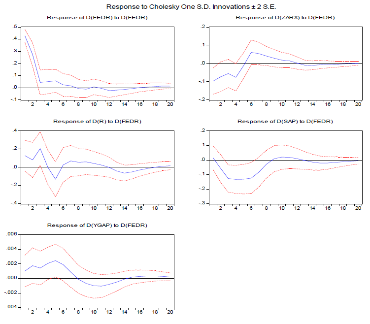
The impulse responses are presented in Figure 2. The dotted lines are one standard error bands computed by Cholesky simulations. Reference [37] posited that the use of one standard deviation bands is advantageous in that makes it easy to compare the findings of the research with other research findings. The impulse responses were calculated over 20 periods which is equal to a period of 5 years. From Figure 2, a positive shock to the US federal funds rate (FedR) (contractionary monetary policy) results in an immediate and statistically significant increase in itself for up to 3 periods after the shock. After the 3 periods, the impact of the shock becomes statistically insignificant. The South African 91 day T Bill rate (R) shows a statistically significant and positive response of 0.21 per cent to a positive shock in the US federal funds rate only in period 3. The response is statistically insignificant in all other periods. The increase in the interest rate is consistent with the findings of [6] [7] along with [37] . It can be explained as the SARB’s attempt to suppress capital outflows in light of an increase in US interest rates or a general increase in world interest rates following contractionary monetary policy in the US due to the size and importance of the US economy in the global space. Moreover, according to [45] , around 93 per cent of South Africa’s total foreign debt is denominated in US Dollar and the Euro. Therefore, an increase in domestic rates following an increase in the US federal funds rate

Figure 2. Impulse responses to US federal funds rate shock under Cholesky ordering: D(FEDR) D(YGAP) D(SAP) D(R) D(ZARX).

could be understood as an attempt to keep the real cost of the foreign debt from rising following an appreciation of the US Dollar.

Figure 2 shows that South African inflation responds negatively to a positive shock in the US federal funds rate from period 3 to period 6, after which the impact becomes statistically insignificant. According to [4] , this can be reflective of a direct deflationary effect that corresponds to deflation in the US and in world commodity prices coupled with a domestic tightening of monetary policy. The response of the Rand-US Dollar exchange rate to a positive shock in the US federal funds rate is negative and statistically significant only in period 1. After that time, the response becomes statistically insignificant. This shows an appreciation of the South African Rand against the US Dollar and ties well with the short-term increase in interest rates observed earlier. It is also complemented by the findings of [31] . Last, the impulse response of the South African output gap to a positive shock in the US federal funds rate is positive in period 5, meaning an increase in actual output over expected levels. These findings align well with the positive interest rate response seen in period 3 as well as the Rand appreciation seen in period 1 given that [6] and [31] discovered that an inflow of foreign capital, which raises the demand for domestic currency, was found to boost domestic production.

5.5. Forecast Error Variance Decomposition

Forecast error variance decompositions are another way of investigating the effect of nonzero residuals (or shocks) in a VAR system. Reference [32] pointed out that variance decompositions can be used as tools to determine the importance of monetary policy shocks in explaining particular developments in macroeconomic history. Table 5 presents the forecast error variance decompositions¹¹ extracted for the tenth and twentieth quarters. The percentage of variation in the row variables, labelled 1 through 5, is explained by shocks to the column variables, labelled a through e.

Table 5. Forecast error variance decomposition in percentage.

Table 5 shows that the US federal funds rate explains 69.25 per cent of its own variation in the short term and 67.90 per cent in the long run. The South African inflation, 91 day T Bill rate and the Rand-US Dollar exchange rate, respectively account for no more than 8.4 per cent of the variation in the US federal funds rate in the short to long run. The South African output gap on the other hand explains 19.6 per cent of the variation in the US federal funds rate in the short run and 20.5 per cent in the long run. The variance decomposition for the South African output gap shows that the output gap accounts for 75.93 per cent and 74.89 per cent of its own variation in the short run and long run. This is followed by the US federal funds rate that explains 9.39 per cent and 10.19 per cent of its variation in the short run and long run, respectively. Domestic inflation, the 91 day T Bill rate and the Rand-US Dollar exchange rate together account for at most 7.1 per cent of the variation observed in the South African output gap in the short run and long run.

The South African inflation rate explains 49.69 per cent of its own variation in the short run and 49.17 per cent in the long run. This is followed by the output gap that explains 20.91 per cent of the variation in inflation the short run and 20.55 per cent in the long run. The US federal funds rate on the other hand explains 16.79 per cent of the variation in South African inflation in the short run and 16.86 per cent in the long run. The rest of the South African macro variables account for no more than 10 per cent of the variation observed in consumer prices both in the short run and long run, respectively. The South African 91 day T Bill rate that is taken to proxy the domestic monetary policy instrument over the sample period explains 59.5 per cent of its own variation in the short run and 57.7 per cent in the long run. This is followed by the output gap that accounts for 23.3 per cent of the variation in the 91 day T Bill rate in the short run and 23.8 per cent in the long run. The US federal funds rate accounts for 8.3 per cent of the variation in South African 91 day T Bill rate in the short run and 9 per cent in the long run. The remaining South African macro variables explain at most 5 per cent of the variation in the 91 day T Bill rate in the short run and long run, respectively. The variance decomposition for the Rand-US Dollar exchange rate depicts that the greatest variation in the short run and long run is explained by own innovations, followed by shocks to the US federal funds rate, domestic inflation, the 91 day T Bill rate and the domestic output gap, respectively.

6. Robustness Checks

In order to check the robustness of our results, [46] espoused that the first stability condition that all the roots of the characteristic polynomial are inside the unit circle should be satisfied. Appendix 1 provides evidence that all roots of the characteristic polynomial lie within the unit circle and as such the VAR model is stable. A second test for robustness is to estimate equation 1 with a change in the ordering of the endogenous variables in the VAR. This is done to assess the responses of the variables to shocks under the new ordering as well as to establish how similar the resultant responses are to previous responses under the ordering specified in Section 4.5¹². Under the new ordering, the study maintains the use

of the Cholesky decomposition with $\frac{n^2-n}{2}$ zero (exclusion) restrictions and

orders the FedR first, followed by ZARx, R, SAp and lastly Ygap. The assumption is that the US federal funds rate is not contemporaneously affected by South African macro variables whereas South African macro variables are assumed to be contemporaneously affected by shocks in the US federal funds rate. Furthermore, shocks in the US federal funds rate are assumed to first be transmitted to the South African macro variables through the exchange rate channel. The impulse responses of South African macro variables to a shock in the US policy rate are presented in Appendix 5 while the corresponding variance decompositions are presented in Appendix 6. As the results indicate, the impulse responses and variance decompositions remain broadly unchanged. This adds credibility to the robustness of the model used.

The third test for robustness undertaken is to estimate Equation (1) when the variables are mixed in nature (that is, a mix of I(0) and I(1) variables). Under

this test, the use of the Cholesky decomposition with $\frac{n^2-n}{2}$ zero (exclusion)

restrictions is maintained and the ordering is such that the FedR is first, followed by ZARx, R, SAp and lastly Ygap. This time around, the VAR is estimated with 4 lags and the inclusion of a trend. Appendix 8 presents the impulse responses. From the impulse responses the results of the study remain broadly unchanged, adding further credibility to the model the robustness of the model used.

7. Conclusions

This paper investigated the impact of shocks to the US federal funds rate (FedR) on South African output gap (Ygap), consumer prices (SAp), 91-day Treasury bill rate (R) and Rand-US Dollar exchange rate over the first quarter of 1981 to the last quarter of 2014 using an SVAR model. Positive innovations in the US federal funds rate are found to negatively affect domestic inflation between period 3 and period 6 after the initial shock. This could be interpreted as a complementary reaction to corresponding deflation in the US and in world commodity prices. The decline in domestic prices also corresponds to a tightening of domestic monetary policy especially since a positive shock to the US federal funds rate was found to result in a rise of the 91-day T Bill rate by 0.21 per cent in period 3. The rise in the 91-day T Bill rate in this instance testifies to a decision taken by the South African Reserve Bank to quell capital outflows in the short-term and prevent the rise of US Dollar denominated foreign debt given a rise in US interest rates and an appreciation of the US Dollar. Positive innovations in the US federal funds rate were discovered to lead to an appreciation in the South African Rand against the US Dollar in the first quarter after the shock. This reaction results in increased capital inflows and an improvement in central bank reserves. Furthermore, similar to [6] , contractionary US monetary policy provokes an increase in the level of South African output observed in a positive output gap in period 5. Domestic developments appear to play the most significant role in determining the fluctuations of South Africa’s macro-variables as US shocks account for only 10 to 17 per cent of the variability in the selected South African macro-variables. A similar finding was made by [4] . Overall, the results indicate that a positive shock in the US federal funds rate (a contractionary monetary policy) is transmitted mainly through the inflation channel with 17 per cent of the variation in domestic prices explained by changes in the US federal funds rate.

Despite the modest impact of US shocks in explaining South African macroeconomic fluctuations, their influence on South African prices cannot be ignored. This is especially true given that US monetary policy shocks were found to affect South Africa’s domestic inflation the most relative to other domestic macro variables. The policy recommendation is that the SARB has to remain mindful of domestic developments as well as movements in the US federal funds rate so as to determine their upside risks to inflation before deciding on a policy stance. This is crucial, especially in light of the SARB’s inflation targeting monetary policy regime.

Acknowledgements

The author wishes to express his gratitude to Dr. Monaheng Seleteng¹³ and Mr Senei Molapo¹⁴ for their useful inputs and comments in writing this paper.

Appendix

Appendix 1. AR Roots Graph (Roots of Characteristic Polynomial)

Appendix 2. Normality Test

Appendix 3. Heteroskedasticity Test

Appendix 4. Forecast Error Variance Decomposition in Percentage under Cholesky Ordering: D(FEDR) D(YGAP) D(SAP) D(R) D(ZARX)

Appendix 5. Impulse Responses to US Federal Funds Rate Shock under Cholesky Ordering: D(FEDR) D(ZARX) D(R) D(SAP) D(YGAP)

Appendix 6. Forecast Error Variance Decomposition in Percentage under Cholesky Ordering: D(FEDR) D(ZARX) D(R) D(SAP) D(YGAP)

Appendix 7. Johansen Cointegration Test with Intercept (No Trend) in CE and Test VAR

Appendix 8. Impulse Responses to US Federal Funds Rate Shock under Cholesky Ordering: FEDR D(ZARX) D(R) SAP YGAP

NOTES

¹An economic shock is defined as an event that produces a significant change within an economy, despite occurring outside of it.

²Following the general election of 27 April 1994, South Africa transitioned from an Apartheid regime to a system of majority rule. The year 1994 marked 3 years after the US lifted economic sanctions on South Africa.

³The indicators were changes in bank credit extension, other overall liquidity in the banking system, the level of the yield curve, changes in the official foreign reserves and in the exchange rate of the rand; and actual and expected movements in the rate of inflation.

⁴The domestic indicators include, but are not limited to; growth in money supply, growth in bank credit extension, the changes in nominal and real salaries and wages, the nominal unit labour costs, the gap between potential and actual domestic output, exchange rate developments, producer prices and import prices.

⁵The foreign indicators include, but are not limited to; oil prices, food prices and administered prices.

⁶The Consumer Price Index excludes mortgages interest cost for metropolitan and urban areas, known as the CPIX.

⁷The repo rate was introduced on 9 March 1998 to ensure greater response of interest rates to financial market developments [18] .

⁸The output gap is calculated as the difference between the log of real Gross Domestic Product and expected output.

⁹To test for autocorrelation in the residuals, the study proposes the Breusch-Godfrey LM test. According to [33] , this is the most suitable test for checking autocorrelation in low order VARs.

¹⁰Where n is the number of endogenous variables in the model.

¹¹A more detailed variance decomposition table is presented in Appendix 4.

¹²The ordering began with the FedR followed by Ygap, then, SAp, R, and ZARx. Using the Cholesky decomposition, this ordering assumed that the US federal funds rate is not contemporaneously affected by changes in South African macroeconomic variables. Moreover, shocks in US monetary policy contemporaneously affect South African macro variables and are first transmitted through the output channel.

¹³Principal Economist at the Central Bank of Lesotho.

¹⁴Programme Manager at the Macroeconomic and Financial Management Institute of Eastern and Southern Africa.

Conflicts of Interest

The authors declare no conflicts of interest.

References

[1]	Huh, H.S. (1999) How Well Does the Mundell-Fleming Model Fit Australian Data since the Collapse of Bretton Woods? Applied Economics, 31, 397-407. https://doi.org/10.1080/000368499324372
[2]	Friedman, T.L. (2005) The World Is Flat: A Brief History of the Twenty-First Century. Farrar, Straus and Giroux, New York.
[3]	Kamin, S.B. (2010) Financial Globalization and Monetary Policy. FRB International Finance Discussion Paper 1002. https://doi.org/10.2139/ssrn.1657893
[4]	Mackowiak, B. (2001) External shocks, U.S. Monetary Policy and Macroeconomic Fluctuations in Emerging Markets. Journal of Monetary Economics, 54, 2512-2520. https://doi.org/10.1016/j.jmoneco.2007.06.021
[5]	Jacobsson, T., Jansson, P., Vredin, A. and Warne, A. (2002) Identifying the Effects of Monetary Policy Shocks in an Open Economy. European Central Bank, Frankfurt.
[6]	Canova, F. (2005) The Transmission of US Shocks to Latin America. Journal of Applied Econometrics, 20, 229-251. https://doi.org/10.1002/jae.837
[7]	Kronick, J. (2014) Monetary Policy Shocks from the EU and US: Implications for Sub-Saharan Africa. University Library of Munich, Munich.
[8]	Ramos-Francia, M. and García-Verdú, S. (2014) The Transmission of US Monetary Policy Shocks to EMEs: An Empirical Analysis. Bank for International Settlements, Basel.
[9]	Kazi, I.A., Wagan, H. and Akbar, F. (2013) The Changing International Transmission of US Monetary Policy Shocks: Is There Evidence of Contagion Effect on OECD Countries. Economic Modelling, 30, 90-116. https://doi.org/10.1016/j.econmod.2012.07.020
[10]	Vespignani, J.L. and Ratti, R.A. (2016) Not All International Monetary Shocks Are Alike for the Japanese Economy. Economic Modelling, 52, 822-837. https://doi.org/10.1016/j.econmod.2015.10.019
[11]	World Integrated Trade Solution (WITS) (2017) South Africa Trade Summary 2015 Data. http://wits.worldbank.org/CountryProfile/en/Country/ZAF/Year/2015/Summary
[12]	Kim, S. (2001) International Transmission of US Monetary Policy Shocks: Evidence from VAR’s. Journal of Monetary Economics, 48, 339-372. https://doi.org/10.1016/S0304-3932(01)00080-0
[13]	Reside Jr., R.E. (2004) International Transmission of US Monetary Policy Shocks: VAR Evidence from the Philippines. UP School of Economics Discussion Papers 200405, University of the Philippines School of Economics, Quezon City.
[14]	Sims, C.A. (2013) Comment on “A Macroeconomic Framework for Quantifying Systemic Risk” by He and Krishnamurthy. https://bfi.uchicago.edu/sites/default/files/file_uploads/SimsHeKrshnmrthySlides.pdf
[15]	Jarociński, M. and Mackowiak, B. (2016) Granger-Causal-Priority and Choice of Variables in Vector Autoregressions. Review of Economics and Statistics, 99, 319-329. https://doi.org/10.1162/REST_a_00601
[16]	Sims, C.A. (1980) Macroeconomics and Reality. Econometrica, 48, 1-48. https://doi.org/10.2307/1912017
[17]	Bernanke, B.S. and Blinder, A.S. (1992) The Federal Funds Rate and the Channels of Monetary Transmission. The American Economic Review, 82, 901-921.
[18]	Smal, M.M. and De Jager, S. (2001) The Monetary Transmission Mechanism in South Africa. South African Reserve Bank, Pretoria.
[19]	Mboweni, T.T. (2004) The Monetary Policy Framework of South Africa. South African Reserve Bank, Pretoria.
[20]	Aron, J. and Muellbauer, J. (2007) Review of Monetary Policy in South Africa since 1994. Journal of African Economies, 16, 705-744. https://doi.org/10.1093/jae/ejm013
[21]	Stals, C. (1997) Effects of the Changing Financial Environment on Monetary Policy in South Africa. Address to the Annual Dinner of the Economic Society of South Africa, Pretoria Branch, 15.
[22]	Angelis, C., Aziakpono, M.J. and Faure, A.P. (2005) The Transmission of Monetary Policy under the Repo System in South Africa: An Empirical Analysis. South African Journal of Economics, 73, 657-673. https://doi.org/10.1111/j.1813-6982.2005.00045.x
[23]	South African Reserve Bank (SARB) (2016) Monetary Policy Review. https://www.resbank.co.za/Lists/News%20and%20Publications/Attachments/7241/ MPRApr2016.pdf
[24]	Mundell, R. (2001) On the History of the Mundell-Fleming Model. Keynote Speech. International Monetary Fund, Washington DC.
[25]	Grenville, S. (2011) The Impossible Trinity. http://voxeu.org/article/how-can-impossible-trinity-not-apply-east-asia
[26]	Rey, H. (2015) Dilemma Not Trilemma: The Global Financial Cycle and Monetary Policy Independence (No. w21162). National Bureau of Economic Research, Cambridge.
[27]	Obstfeld, M. (2001) International Macroeconomics: Beyond the Mundell-Fleming Model (No. w8369). National Bureau of Economic Research, Cambridge. https://doi.org/10.3386/w8369
[28]	Obstfeld, M. and Rogoff, K. (1995) The Intertemporal Approach to the Current Account. Handbook of International Economics, 3, 1731-1799. https://doi.org/10.1016/S1573-4404(05)80014-0
[29]	Moccero, D.N. (2006) The Intertemporal Approach to the Current Account: Evidence from Argentina. Journal of Applied Economics, XI, 327-353.
[30]	Reside Jr., R.E. (2001) Two Decades of Vector Autoregression (VAR) Modelling. Philippine Review of Economics, 38, 83-121.
[31]	Calvo, G.A., Leiderman, L. and Reinhart, C.M. (1993) Capital Inflows and Real Exchange Rate Appreciation in Latin America: The Role of External Factors. Staff Papers, 40, 108-151. https://doi.org/10.2307/3867379
[32]	Clarida, R. (2001) The Empirics of Monetary Policy Rules in Open Economies (No. w8603). National Bureau of Economic Research, Cambridge. https://doi.org/10.3386/w8603
[33]	Lütkepohl, H. (2011) Vector Autoregressive Models. Springer, Berlin Heidelberg, 1645-1647. https://doi.org/10.1007/978-3-642-04898-2_609
[34]	Dickey, D.A. and Fuller, W.A. (1979) Distribution of the Estimators for Autoregressive Time Series with a Unit Root. Journal of the American Statistical Association, 74, 427-431.
[35]	Dickey, D.A. and Fuller, W.A. (1981) Likelihood Ratio Statistics for Autoregressive Time Series with a Unit Root. Econometrica, 49, 1057-1072. https://doi.org/10.2307/1912517
[36]	Phillips, P.C. and Perron, P. (1988) Testing for a Unit Root in Time Series Regression. Biometrika, 75, 335-346. https://doi.org/10.1093/biomet/75.2.335
[37]	Cushman, D.O. and Zha, T. (1997) Identifying Monetary Policy in a Small Open Economy under Flexible Exchange Rates. Journal of Monetary Economics, 39, 433-448. https://doi.org/10.1016/S0304-3932(97)00029-9
[38]	Granger, C.W. (1986) Developments in the Study of Cointegrated Economic Variables. Oxford Bulletin of Economics and Statistics, 48, 213-228. https://doi.org/10.1111/j.1468-0084.1986.mp48003002.x
[39]	Sims, C.A., Stock, J.H. and Watson, M.W. (1990) Inference in Linear Time Series Models with Some Unit Roots. Econometrica, 58, 113-144. https://doi.org/10.2307/2938337
[40]	Khan, M.A.R. and Ali, M.A. (2003) VAR Modeling with Mixed Series. International Journal of Statistical Sciences, 2, 19-26.
[41]	Johansen, S. (1991) Estimation and Hypothesis Testing of Cointegration Vectors in Gaussian Vector Autoregressive Models. Econometrica, 59, 1551-1580. https://doi.org/10.2307/2938278
[42]	Mukherjee, T.K. and Naka, A. (1995) Dynamic Relations between Macroeconomic Variables and the Japanese Stock Market: An Application of a Vector Error Correction Model. Journal of Financial Research, 18, 223-237. https://doi.org/10.1111/j.1475-6803.1995.tb00563.x
[43]	Herrera, A.M. and Pesavento, E. (2013) Unit Roots, Cointegration and Pre Testing in VAR Models. Advances in Econometrics, 32, 81-115. https://doi.org/10.1108/S0731-9053(2013)0000031003
[44]	Marcet, A. (2005) Overdifferencing VARs Is OK. Universitat Pompeu Fabra, Barcelona.
[45]	National Treasury (2016) South African Debt Management Report 2015/16. http://www.treasury.gov.za/publications/other/Debt%20Management% 20Report%202015-16.pdf
[46]	Ravnik, R. and Zilic, I. (2011) The Use of SVAR Analysis in Determining the Effects of fiscal Shocks in Croatia. Financial Theory and Practice, 35, 25-58.