New Class of Distortion Risk Measures and Their Tail Asymptotics with Emphasis on VaR ()
1. Introduction
A risk measure
is a mapping from the set of random variables
, standing for risky portfolios of assets and/or liabilities, to the real line R. In the subsequent discussion, positive values of elements of
will be considered to represent losses, while negative values will represent gains. Distortion risk measures are a particular and most important family of risk measures that have been extensively used in finance and insurance as capital requirement and principles of premium calculation for the regulator and supervisor. Several popular risk measures belong to the family of distortion risk measures. For example, the value-at-risk (VaR), the tail value-at-risk (TVaR) and the Wang distortion measure. Distortion risk measures satisfy a set of properties including positive homogeneity, translation invariance and monotonicity. When the associated distortion function is concave, the distortion risk measure is also subadditive (Denneberg, 1994; Wang & Dhaene, 1998) . VaR is one of the most popular risk measures used in risk management and banking supervision due to its computational simplicity and for some regularity reasons, despite it has some shortcomings as a risk measure. For example, VaR is not a subadditive risk measure (see, for instance, Artzner et al., 1999; Denuit et al., 2005 ), it only concerns about the frequency of risk, but not the size of risk. TVaR, although being coherent, concerns only losses exceeding the VaR and ignores useful information of the loss distribution below VaR. Clearly, it is difficult to believe that a unique risk measure could capture all characteristics of risk, so that an ideal measure does not exist. Moreover, since risk measures associate a single number to a risk, as a matter of fact, they cannot exhaust all the information of a risk. However, it is reasonable to search for risk measures which are ideal for the particular problem under investigation. As all the proposed risk measures have drawbacks and limited applications, the selection of the appropriate risk measures continues to be a hot topic in risk management.
Zhu & Li (2012) introduced and studied the tail distortion risk measure which was reformulated by Yang (2015) as follows. For a distortion function g, the tail distortion risk measure at level p of a loss variable X is defined as the distortion risk measure with distortion function
Some properties and applications can be found in Mao, Lv, & Hu (2012) , Mao & Hu (2013) and Lv, Pan, & Hu (2013) .
As an extension of VaR and TVaR, Belles-Sampera et al. (2014a) proposed a new class of distortion risk measures called GlueVaR risk measures, which can be expressed as a combination of VaR and TVaR measures at different probability levels. They obtain the analytical closed-form expressions for the most frequently used distribution functions in financial and insurance applications, while a subfamily of these risk measures has been shown to satisfy the tail-subadditivity property which means that the benefits of diversification can be preserved, at least they hold in extreme cases. The applications of GlueVaR risk measures in capital allocation can be found in the recent paper Belles-Sampera et al. (2014b) .
Cherubini & Mulinacci (2014) propose a class of distortion measures based on contagion from an external “scenario” variable. The dependence between the scenario and the variable whose risk is modeled with a copula function with horizontal concave sections, they give conditions to ensure that coherence requirements be met, and propose examples of measures in this class based on copula functions.
The first purpose of this paper is to construct new risk measures following Zhu & Li (2012) , Belles-Sampera et al. (2014a) and Cherubini & Mulinacci (2014) . The newly introduced risk measures are included the tail distortion risk measure and the GlueVaR as specials. The second goal of the paper is to investigate the tail asymptotics of distortion risk measures for the sum of possibly dependent risks with emphasis on VaR. The rest of the paper is organized as follows. We review some basic definitions and notations such as distorted functions, distorted expectations and distortion risk measures in Section 2. In Section 3 several new distortion functions and risk measures are introduced. In Section 4 we investigate the tail asymptotics as well as subadditivity/superadditivity of VaR. In Section 5 we analyze the subadditivity properties of a class of distortion risk measures and Section 6 focuses on conclusion.
2. Distortion Risk Measures
2.1. Distorted Functions
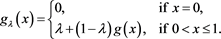
A distortion function is a non-decreasing function
such that
. Since Yaari (1987) introduced distortion function in dual theory of choice under risk, many different distortions g have been proposed in the literature. Here we list some commonly used distortion functions. A summary of other proposed distortion functions can be found in Denuit et al. (2005) .
•
, where the notation
to denote the indicator function, which equals 1 when A holds true and 0 otherwise.
•
.
・ Incomplete beta function
, where
and
are parameters and
. Setting
gives the power distortion
; setting
gives the dual-power distortion
.
・ The Wang distortion
, where
is the distribution function of the standard normal.
・ The lookback distortion
Obviously, every concave distortion function is continuous on the interval
and can have jumps in 0. In contrast, every convex distortion function is continuous on the interval
and can have jumps in 1. The identity function is the smallest concave distortion function and also the largest convex distortion function;
is concave on
and is the largest distortion function.
is convex on
and is the smallest
distortion function. For
, we remark that
is
the smallest concave distortion function such that
. In fact, we consider a concave distortion function g such that
, then
on
. As g is concave, it follows that
for
, and thus
for
. Any concave distortion function g
gives more weight to the tail than the identity function
, whereas any convex distortion function g gives less weight to the tail than the identity function
.
2.2. Distorted Risk Measures
Let
be a probability space on which all random variables involved are defined. Let
be the cumulative distribution function of random variable X and the decumulative distribution function is denoted by
, i.e.
. Let g be a distortion function. The distorted expectation of the random variable X, notation
, is defined as
provided at least one of the two integrals above is finite. If X a non-negative random variable, then
reduces to
From a mathematical point of view, a distortion expectation is the Choquet integral (see Denneberg (1994) ) with respect to the nonadditive measure
. That is
. In view of Dhaene et al. (2012: Theorems 4 and 6) we know that, when the distortion function g is right continuous on
, then
may be rewritten as
where
, and when the distortion function g is left continuous on
, then
may be rewritten as
where
and
is the dual distortion of g. Obviously,
, g is left continuous if and only if
is right continuous; g is concave if and only if
is convex. The distorted expectation
is called a distortion risk measure with distortion function g. Distortion risk measures are a particular class of risk measures which as premium principles were introduced by Denneberg (1994) and further developed by Wang (1996, 2000) among others.
Distortion risk measures satisfy a set of properties including positive homogeneity, translation invariance and monotonicity. A risk measure is said to be coherent if it satisfies the following set of four properties (see, e.g., Artzner et al., 1997, 1999 ):
(M) Monotonicity:
provided that
.
(P) Positive homogeneity: For any positive constant
and loss X,
.
(S) Subadditivity: For any losses
, then
.
(T) Translation invariance: If c is a constant, then
.
It is furthermore shown by Artzner et al. (1999) that all mappings satisfying the above properties allow a representation:
where
is a collection of “generalised scenarios”. A risk measure
is called a convex risk measure if it satisfies monotonicity, translation invariance and the following convexity (C):
Clearly, under the assumption of positive homogeneity, monotonicity and translation invariance, the convexity of a risk measure is equivalent subadditivity.
The most well-known examples of distortion risk measures are the above-mentioned VaR and TVaR, corresponding to the distortion functions,
respectively, are
and
. Notice that
can be alternatively expressed as the weighted average of VaR and losses exceeding VaR:
(2.1)
For continuous distributions, TVaR coincide with the expected loss exceeding p-Value-at Risk, i.e., the mean of the worst
losses in a specified time period which defined by
Detailed studies of distortion risk measures and their relation with orderings of risk and the concept of comonotonicity can be found in, for example, Wang (1996) , Wang & Young (1998) , Hua & Joe (2012) and the references therein. The following lemma will be used in proofs of later results, which characterizes an ordering of distortion risk measures in terms of their distortion functions.
Lemma 2.1 (Belles-Sampera et al., 2014b) . If
for
, then
for any random variable X.
3. Generating New Distortion Functions and Measures
Distortion functions can be considered as a starting point for constructing families of distortion risk measures. Thus, constructions of distortion functions play an important role in producing various families of risk measures. Using the technique of mixing, composition and copula allow the construction of new class of distortion functions and measures.
3.1. Composting Methods
The first approach to construct distortion functions is the composition of distortion functions.
Let
be distortion functions, define
and composite functions
. It is easy to check that
are all distortion functions. If
are concave distortion functions, then each
is concave and satisfies that
and
The associated risk measures satisfy (by Lemma 2.1)
and
If
are convex distortion functions, then each
is convex and satisfies that
and
The associated risk measures satisfy (by Lemma 2.1)
and
Consider two distortion functions
and
. If
then we get
The corresponding risk measure
is the tail distortion risk measure which was first introduced by Zhu & Li (2012) , and was reformulated by Yang (2015) . In particular, on the space of continuous loss random variables X,
If
and
then
and
Clearly,
and
, so that, by Lemma 2.1,
and
.
In practice, sometimes one needs distort the initial distribution more than one times.
Example 3.1 Consider two risks X and Y with distributions, respectively, are:
and
Then
,
,
.
TVaR can be calculated by formula (2.1):
,
. So that when
and
, according to the measures of VaR and TVaR, both X and Y bear the same risk! However, the maximal loss for Y (1100) is more than double than for loss X (500), clearly, risk Y is more risky than risk X. Now we consider distortion expectation
with
One can easily find that, with
,
and
.
3.2. Mixing Methods
One of the easiest ways to generate distortion functions is to use the method of mixing along with finitely distortion functions or infinitely many distortion functions. Specifically, if
(
) is a one-parameter family of distortion functions,
is an increasing function on
such that
, then the function
is a distortion function,
the associated risk measure is given by
(3.1)
In particular, if
is discrete distribution, then (3.1) can be written as the form of convex linear combination
, the associated risk measure is given by
(3.2)
Further studies on this line can be found recent papers He et al. (2015) and Wei (2017) .
The following lemma is well known (cf. Kriele & Wolf (2014: Theorem 2.1, p. 33) ).
Lemma 3.1 If all
(
) are monotone, positively homogeneous, subadditive and translation invariant, then
also has the corresponding properties. That is, if all
(
) are coherent, then
is also coherent.
Now we list three interesting special cases:
If
,
and
, then v in (3.2) is coherent since
is concave. As in Tsukahara (2009) , if we take
from Bin v (
), then
. If we take
then
Also, if we take
(
), the geometric distribution, then
which is the proportional odds distortion; see Example 2.1 in Cherubini & Mulinacci (2014) .
If
,
and
, then
in (3.1) reduces to
(3.3)
which is spectral risk measure (see Acerbi, 2002 ). Here
is called a
weighting function satisfies the following properties:
,
. The
following lemma gives a sufficient condition for
to be a coherent risk measure (cf. Kriele & Wolf (2014) ).
Lemma 3.2 Spectral risk measure
is coherent if
is (almost everywhere) monotone increasing.
Clearly, there exists a one-to-one correspondence between distortion function g and weighting function
, namely,
If
,
and
is a probability measure on
, then
in (3.1) reduces to
(3.4)
which is the weighted TVaR (see Cherny (2006) ).
is a special weighted TVaR with
. According to Lemma 3.1, since each
is coherent risk measure, the weighted TVaR is coherent risk measure. The weighted TVaR can be rewritten as the form of spectral risk measure as following:
where g is a function with
and satisfies
Because
is increasing function of q, it follows from Lemma 3.2 that the weighted TVaR
is coherent. Or, equivalently,
is decreasing function of q, i.e. g is a concave function, moreover, g is increasing and
so that g is a concave distortion function, and hence the weighted TVaR is coherent.
Conversely, the distortion measure with concave distortion function g can be expressed by the weighted TVaR. In fact, note that
is monotone increasing, we define a measure
. As in the proof of Theorem 2.4 in Kriele & Wolf (2014) we have
where
It can be shown that
is a probability measure. In fact,
We now give some examples of interesting distortion functions and risk measures.
Example 3.2 If
, then
is a distortion function, where
are the distortion functions of TVaR and VaR at confidence levels  and
and , respectively. Then the corresponding risk measure

is called the GlueVaR risk measure, which were initially defined by Belles-Sampera et al. (2014a) (in the case ) and the closed-form expressions of GlueVaR for Normal, Log-normal, Student’s t and Generalized Pareto distributions are provided. Two new proportional capital allocation principles based on GlueVaR risk measures are studied in Belles-Sampera et al. (2014b) .
Although GlueVaR has superior mathematical properties than VaR and TVaR, however, the GlueVaR risk measure may also fails to recognize the differences between two risks. For example, consider two risks X and Y in Example 3.1, we have computed that ,
,  .
. ,
,  . So that when
  and
and , we have
 . Thus according to
 , both X and Y bear the same risk! However, the maximal loss for Y (1100) is more than double than for loss X (500), clearly, risk Y is more risky than risk X.
Example 3.3 Let , define a distortion function

where  and g is an arbitrary distortion function. Note that
  can be rewritten as
In particular, if , then we get the esssup-expectation convex combination distortion function with weight
 ![]() on the essential supremum, which was introduced in Bannör & Scherer (2014) . The corresponding risk measure
on the essential supremum, which was introduced in Bannör & Scherer (2014) . The corresponding risk measure
![]()
which is a convex combination of the essential supremum of X and the ordinary expectation of X w.r.t. P.
If
![]()
where![]() ,
, ![]() are constants, then we get
are constants, then we get
![]()
where
![]()
As illustration, we consider the risks X and Y in Example 3.1, if![]() , then
, then![]() . It follows that
. It follows that
![]()
and
![]()
Taking![]() , then
, then ![]() and
and![]() . Taking
. Taking![]() , then
, then ![]() and
and![]() . Thus
. Thus ![]() can measure the differences between two risks X and Y.
can measure the differences between two risks X and Y.
3.3. A Copula-Based Approach
If F is a distribution function on![]() , then F can be used as a distortion function. The well-known examples are the PH transform and the dual power transform and, more generally, the beta transform; see Wirch & Hardy (1999) for details. Similarly, we use this technique to a distribution function on
, then F can be used as a distortion function. The well-known examples are the PH transform and the dual power transform and, more generally, the beta transform; see Wirch & Hardy (1999) for details. Similarly, we use this technique to a distribution function on![]() . We first introduce the notion of copula in the two-dimensional case.
. We first introduce the notion of copula in the two-dimensional case.
Definition 3.1. A two-dimensional copula ![]() is a bivariate distribution on the square
is a bivariate distribution on the square ![]() having uniform margins. That is a function
having uniform margins. That is a function ![]() is right-continuous in each variable such that
is right-continuous in each variable such that![]() ,
, ![]() ,
, ![]() and for
and for![]() ,
,
![]()
For an introduction to copula theory and some of its applications, we refer to Joe (1997) , Denuit et al. (2005) and Nelsen (1999) .
The well-known examples of copulas are![]() ,
, ![]() and
and ![]() describing, respectively, comonotone dependence, independence and countermonotone dependence between two random variables X and Y. The copula version of the Fréchet-Hoeffding bounds inequality tells us
describing, respectively, comonotone dependence, independence and countermonotone dependence between two random variables X and Y. The copula version of the Fréchet-Hoeffding bounds inequality tells us
![]()
Any copula has the following decomposition (cf. Yang et al. (2006) )
![]()
where![]() ,
,![]() . Here G is a copula which called the indecomposable part.
. Here G is a copula which called the indecomposable part.
For a given two-dimensional copula![]() , define one-parameter family
, define one-parameter family
![]() by
by ![]() or
or![]() . Clearly, for each p,
. Clearly, for each p, ![]() is a right
is a right
continuous distortion function. For example,
• ![]() is continuous and both convex and concave, the associated risk measure is
is continuous and both convex and concave, the associated risk measure is![]() ;
;
• ![]() is continuous and concave, the corresponding risk measure is
is continuous and concave, the corresponding risk measure is![]() ;
;
• ![]() is continuous and convex, the corresponding risk measure is
is continuous and convex, the corresponding risk measure is![]() .
.
Conversely, if ![]() is a family of distortion functions, then, however,
is a family of distortion functions, then, however, ![]() is not a copula in general; A sufficient condition can be found in Cherubini & Mulinacci (2014) .
is not a copula in general; A sufficient condition can be found in Cherubini & Mulinacci (2014) .
We give below the most common bivariate copulas and the corresponding distortion functions.
• The Archimedean copulas:
![]()
for some generator ![]() with
with ![]() such that
such that ![]() is convex. The pseudo-inverse of
is convex. The pseudo-inverse of ![]() is the function
is the function ![]() with
with ![]() and
and ![]() given by
given by
![]()
If ![]() is twice differentiable and
is twice differentiable and![]() , then
, then ![]() is componentwise
is componentwise
concave if, and only if ![]() is concave, where
is concave, where ![]() is the derivative of
is the derivative of ![]() (see
(see
Dolati & Nezhad (2014) ). Aa a consequence, we have
Theorem 3.1 For each![]() , the distortion function
, the distortion function
![]()
is concave if, and only if ![]() is concave.
is concave.
Some examples of the Archimedean copulas and the corresponding distortion functions:
a) The Clayton copula with parameter ![]() is generated by
is generated by ![]() and takes the form
and takes the form
![]()
The limit of ![]() for
for ![]() and
and ![]() leads to independence and comonotonicity respectively (Nelsen, 1999) . The corresponding distortion functions are
leads to independence and comonotonicity respectively (Nelsen, 1999) . The corresponding distortion functions are
![]()
In particular, if![]() , we get the proportional odds distortion which is found by Cherubini & Mulinacci (2014) :
, we get the proportional odds distortion which is found by Cherubini & Mulinacci (2014) :
![]()
Since![]() ,
, ![]() is concave.
is concave.
b) In case![]() , we get the Frank copulas:
, we get the Frank copulas:
![]()
The corresponding distortion functions are
![]()
Since![]() ,
, ![]() is convex if
is convex if ![]() and concave if
and concave if![]() .
.
c) In case![]() , we get the Pareto survival copulas:
, we get the Pareto survival copulas:
![]()
The corresponding distortion functions are
![]()
Since![]() ,
, ![]() is concave.
is concave.
d) In case![]() , we get the Ali-Mikhail-Haq copulas:
, we get the Ali-Mikhail-Haq copulas:
![]()
The corresponding distortion functions:
![]()
Since![]() ,
, ![]() is convex if
is convex if ![]() and concave if
and concave if![]() .
.
e) In case![]() , we get the Gumbel-Hougaard copulas:
, we get the Gumbel-Hougaard copulas:
![]()
The corresponding distortion functions:
![]()
The value ![]() gives independence and the limit for
gives independence and the limit for ![]() leads to comonotonicity. Since
leads to comonotonicity. Since
![]()
![]() is concave if
is concave if ![]() and, if
and, if![]() ,
, ![]() is convex on
is convex on ![]() and concave on
and concave on![]() .
.
Among other copulas, which do not belong to Archimedean family, it is worth to mention the following three copulas, given in the bivariate case as:
• The Farlie-Gumbel-Morgenstern copulas:
![]()
The corresponding distortion functions are
![]()
which is convex if ![]() and concave if
and concave if![]() .
.
• The Marshall-Olkin copulas:
![]()
Note that this copula is not symmetric for![]() . The corresponding distortion functions are
. The corresponding distortion functions are
![]()
which is concave. In particular, ![]() ,
,
![]()
• The normal copulas:
![]()
where ![]() is a bivariate normal distribution with standard normal marginal distributions and the correlation coefficient
is a bivariate normal distribution with standard normal marginal distributions and the correlation coefficient![]() ,
, ![]() is the inverse function of the standard normal distribution. The corresponding distortion functions:
is the inverse function of the standard normal distribution. The corresponding distortion functions:
![]()
4. Tail-Asymptotics for VaR
Subadditivity is an appealing property when aggregating risks in order to preserve the benefits of diversification. Subadditivity of two risks is not only dependent on their dependence structure but also on the marginal distributions. Value at risk is one of the most popular risk measures, but this risk measure is not always subadditive, nor convex, exception of elliptically distributed risks. This family consists of many symmetric distributions such as the multivariate normal family, the multivariate Student-t family, the multivariate logistic family and the multivariate exponential power family, and so on. A recent development in the VaR literature concerns the subadditivity in the tails (see Daníelsson et al. (2013) ) which demonstrate that VaR is subadditive in the tails of all fat tailed distributions, provided the tails are not super fat. However, in most practical models of interest the support of loss is bounded so that the maximum loss is simply finite. We will also show that for this class losses VaR is subadditive in the tail. We can illustrate the ideas here with three simple examples. In Examples 4.1 and 4.3, X and Y are independent, while in Example 4.2, X and Y are dependent.
Example 4.1 Let X and Y be i.i.d. random variables which are Bernoulli (0.02) distributed, i.e.![]() . Then
. Then
![]()
![]()
![]()
Dhaene et al. (2006) verified that VaR is not subadditive since ![]() and
and![]() . However, for
. However, for![]() ,
, ![]() and
and
![]()
Thus for![]() ,
,
![]()
Example 4.2 Suppose we have losses X and Y, both dependent on the same underlying Uniform (0,1) random variable U as follows.
![]()
![]()
Note that
![]()
![]()
Hardy (2006) found that![]() ,
,![]() . Thus
. Thus
![]()
However, for any![]() ,
, ![]() ,
, ![]() . Thus,
. Thus,
![]()
Example 4.3 Let X and Y be i.i.d. random variables which are Uniform (0,1) distributed. Then
![]()
and for![]() ,
, ![]() ,
,
![]()
Thus for![]() ,
,
![]()
Generally, we have the following result.
Theorem 4.1 If the risks ![]() have finite upper endpoints, then
have finite upper endpoints, then
![]()
Proof The proof is very simple. Denote by![]() . Then
. Then ![]() and
and![]() , which lead to
, which lead to
![]()
Hence
![]()
and the result follows.
Next theorem consider the random variables ![]() that are not necessarily has finite upper endpoint, we first recall the notion of (extended) regularly varying function:
that are not necessarily has finite upper endpoint, we first recall the notion of (extended) regularly varying function:
Definition 4.1 A function f is called regularly varying at some point ![]() (or
(or![]() , respectively) with index
, respectively) with index ![]() if for all
if for all![]() ,
,
![]()
(or![]() , respectively). We write
, respectively). We write ![]() (
(![]() , respectively). For
, respectively). For ![]() we say f is slowly varying; for
we say f is slowly varying; for ![]() rapidly varying.
rapidly varying.
Definition 4.2 Assume that F is the distribution function of a nonnegative random. We say F belongs to the extended regular variation class, if there are some ![]() such that
such that
![]()
or equivalently
![]()
We write![]() .
.
A standard reference to the topic of (extended) regular variation is Bingham et al. (1987) while main results are summarized by Embrechts et al. (1997) .
Theorem 4.2 We assume that ![]() have the same absolutely continuous marginal distributions F with infinite upper endpoint.
have the same absolutely continuous marginal distributions F with infinite upper endpoint.
1) If
![]() (4.1)
(4.1)
then
![]() (4.2)
(4.2)
(2) If
![]()
then
![]()
3) If
![]()
then
![]()
Proof We prove (1) only since the other cases follow immediately in the same way. Because all the marginal distributions are absolutely continuous, so we have for any![]() ,
,
![]()
This, together with (4.1), implies that
![]() (4.3)
(4.3)
The absolute continuity of F implies that ![]() is continuous and strictly monotone decreasing. Then from (4.3) we have
is continuous and strictly monotone decreasing. Then from (4.3) we have
![]()
which is (4.2). This completes the proof.
Example 4.4 Suppose that each ![]() is regularly varying with index
is regularly varying with index![]() . When the
. When the ![]() are mutually independent, it follows from (Feller, 1971: p. 279) that
are mutually independent, it follows from (Feller, 1971: p. 279) that
![]()
Thus we get
![]()
Suppose that the ![]() are comonotonic, i.e.
are comonotonic, i.e.![]() , then
, then
![]()
So that in the case ![]() the result for the independent and the comonotonic case are the same.
the result for the independent and the comonotonic case are the same.
The following result generalizes the result in Jang & Jho (2011) in which all ![]() ‘s are assumed identically distributed.
‘s are assumed identically distributed.
Theorem 4.3 Suppose ![]() are nonnegative random variables (but not necessarily independent or identically distributed.) If
are nonnegative random variables (but not necessarily independent or identically distributed.) If ![]() has distribution F satisfying
has distribution F satisfying![]() , where
, where ![]() is slowly varying at
is slowly varying at
infinity. If ![]() and
and![]() , as
, as![]() ,
, ![]() , then
, then
![]()
Proof It follows from Lemma 2.1 in Davis & Resnick (1996) that
![]()
This leads to
![]() (4.4)
(4.4)
Because
![]()
Thus from (4.4) that
![]()
which is equivalent to
![]()
This implies that
![]()
since ![]() is continuous and strictly monotone decreasing. Note that
is continuous and strictly monotone decreasing. Note that![]() ,
, ![]() (as
(as![]() ) and
) and
![]()
completing the proof.
Remark 4.1 The above result is obtained by Embrechts et al. (2009) for identically distributed and Archimedean copula dependent ![]() ‘s. However, our result can not obtained from their’s due to the following fact: The famous Farlie-Gumbel-Morgenstern family, does not belong to Archimedean family, which has the form
‘s. However, our result can not obtained from their’s due to the following fact: The famous Farlie-Gumbel-Morgenstern family, does not belong to Archimedean family, which has the form
![]()
where ![]() are two distributions and
are two distributions and ![]() is a constant. When
is a constant. When
![]() , it satisfying
, it satisfying ![]() as
as![]() .
.
In the next theorem we consider the extended regularly varying instead of regularly varying.
Theorem 4.4 Suppose ![]() are nonnegative random variables with the common identical distribution function F. If
are nonnegative random variables with the common identical distribution function F. If ![]() and
and
![]() , as
, as![]() ,
, ![]() , then
, then
1) If![]() ,
,
![]()
2) If![]() ,
,
![]()
3) If![]() ,
,
![]()
Proof It follows from Lemma 2.2 in Zhang et al. (2009) that
![]()
This leads to
![]()
from which and using the same argument as that in the proof of Theorem 4.3 leads to
![]() (4.51)
(4.51)
If![]() , then
, then
![]()
This and (4.5) imply that
![]()
It follows that
![]() (4.6)
(4.6)
Thus
![]()
Similarly, if![]() ,
,
![]() (4.7)
(4.7)
and hence
![]()
If![]() , then by (4.6) and (4.7) one has
, then by (4.6) and (4.7) one has
![]() (4.8)
(4.8)
This ends the proof of Theorem 4.4.
To give applications of our results we employ extreme value theory techniques. A distribution function F (or the rv X) is said to belong to the Maximum Domain of Attraction (MDA) of the extreme value distribution H if there exist
constants ![]() such that
such that![]() . We
. We
write ![]() or
or![]() . According to the Fisher-Tippett theorem (see Theorem 3.2.3 in Embrechts et al. (1997) ) H belongs to one of the three standard extreme value distributions:
. According to the Fisher-Tippett theorem (see Theorem 3.2.3 in Embrechts et al. (1997) ) H belongs to one of the three standard extreme value distributions:
![]()
![]()
![]()
Let ![]() denote the right-endpoint of the support of F:
denote the right-endpoint of the support of F:![]() . Then we have the following results (see Embrechts et al. (1997: pp. 132-157) ).
. Then we have the following results (see Embrechts et al. (1997: pp. 132-157) ).
• Fréchet case: For some![]() ,
,![]() .
.
Examples are Pareto, Cauchy, Burr, Loggamma and Stable with index![]() .
.
• Weibull case: For some![]() ,
, ![]() ,
, ![]() .
.
Examples are Uniform and Beta distribution.
• Gumbel case: ![]() and there exists a positive measurable function a such that for
and there exists a positive measurable function a such that for ![]()
![]() (4.9)
(4.9)
Examples are Exponential-like, Weibull-like, Gamma, Normal, Lognormal, Benktander-type-I and Benktander-type-II.
Remark 4.2 1) For![]() , if
, if![]() , in view of Weibull case above they are all have finite supports. It follows from Theorem 4.1,
, in view of Weibull case above they are all have finite supports. It follows from Theorem 4.1, ![]() is subadditive for p is sufficiently close to 1.
is subadditive for p is sufficiently close to 1.
2) For![]() , if
, if ![]() and are identically distributed,
and are identically distributed, ![]() has an Archimedean copula with generator
has an Archimedean copula with generator![]() , which is regularly varying at 0 with index
, which is regularly varying at 0 with index![]() . We apply (2.2) in Alink et al. (2004) and Definition 4.1 to obtain
. We apply (2.2) in Alink et al. (2004) and Definition 4.1 to obtain
![]()
where in the last step we have used Lemma 3.1(d) in Embrechts et al. (2009) which states that
![]()
This, together with Theorem 4.2 we recover the result Theorem 2.5 in Embrechts et al. (2009) .
3) If ![]() have common distribution F,
have common distribution F, ![]() has an Archimedean copula with generator
has an Archimedean copula with generator![]() , which is regularly varying at 0 with index
, which is regularly varying at 0 with index![]() . We apply (2.6) in Alink et al. (2004) to obtain
. We apply (2.6) in Alink et al. (2004) to obtain
![]()
where
![]()
The constant ![]() is strictly increasing in
is strictly increasing in ![]() with
with
![]()
For more details, see Alink et al. (2004) for the case ![]() and Chen et al. (2012) for general case. Thus by Theorem 4.2,
and Chen et al. (2012) for general case. Thus by Theorem 4.2,
![]()
In particular, when![]() ,
,
![]()
5. Tail-Subadditivity for Distortion Risk Measures
The tail-subadditivity property for GlueVaR risk measures were initially defined by Belles-Sampera et al. (2014a) and the milder condition of subadditivity in the tail region is investigated. Furthermore, they verified that a GlueVaR risk measure is tail-subadditive if its associated distortion function ![]() is concave in
is concave in![]() , where parameters
, where parameters ![]() is confidence level and
is confidence level and ![]() is an extra confidence level such that
is an extra confidence level such that ![]() and,
and,
![]()
where ![]() and
and ![]() are two distorted survival probabilities at levels
are two distorted survival probabilities at levels ![]() and
and![]() , respectively. Here
, respectively. Here![]() . We note, however, from their proof to Theorem 6.1 that the result will hold for any distortion function that is concave in
. We note, however, from their proof to Theorem 6.1 that the result will hold for any distortion function that is concave in![]() , not restricted to
, not restricted to![]() . In this section we state the corresponding result without proof. As in Belles-Sampera et al. (2014a) , for a given confidence level
. In this section we state the corresponding result without proof. As in Belles-Sampera et al. (2014a) , for a given confidence level![]() , the tail region of a random variable Z is defined as
, the tail region of a random variable Z is defined as![]() , where
, where ![]() is the a-quantile. For simplicity, we use the notation
is the a-quantile. For simplicity, we use the notation![]() .
.
Theorem 5.1 For a confidence level ![]() and two risks
and two risks ![]() defined on the same probability space. If
defined on the same probability space. If ![]() and g is a concave distortion function in
and g is a concave distortion function in![]() , then the distortion risk measure
, then the distortion risk measure ![]() is tail-subadditive. That is
is tail-subadditive. That is
![]()
where ![]()
Example 5.1 Consider the distortion functions associated with the Gumbel-Hougaard copulas (cf. Section 3.3):
![]()
If![]() , then
, then ![]() is concave on
is concave on ![]() and convex on
and convex on![]() . Thus the distortion risk measure
. Thus the distortion risk measure ![]() is tail-subadditive.
is tail-subadditive.
6. Conclusion
In this paper, we give three methods to construct new class of distortion functions and distortion risk measures and then we investigate the tail asymptotics of distortion risk measures for the sum of possibly dependent risks with emphasis on VaR. We study the concept of tail subadditivity for distortion risk measures and give sufficient conditions for a distortion risk measure to be tail subadditive. The multivariate tail distortion risk measure and more applications of the risk measure will be investigated in the coming research.
Acknowledgements
We thank the anonymous reviewers for their comments. The research was supported by the National Natural Science Foundation of China (11171179, 11571198) and the Research Fund for the Doctoral Program of Higher Education of China (20133705110002).
Author Contributions
Two authors contributed equally to this work.
Conflicts of Interest
The authors declare no conflict of interest.