Iterative Reweighted l₁ Penalty Regression Approach for Line Spectral Estimation

Fei Ye, Xian Luo, Wanzhou Ye

College of Science, Shanghai University, Shanghai, China.

DOI: 10.4236/apm.2018.82008                

Abstract

In this paper, we proposed an iterative reweighted l₁ penalty regression approach to solve the line spectral estimation problem. In each iteration process, we first use the ideal of Bayesian lasso to update the sparse vectors; the derivative of the penalty function forms the regularization parameter. We choose the anti-trigonometric function as a penalty function to approximate the l₀  norm. Then we use the gradient descent method to update the dictionary parameters. The theoretical analysis and simulation results demonstrate the effectiveness of the method and show that the proposed algorithm outperforms other state-of-the-art methods for many practical cases.

Keywords

Line Spectral Estimation, Penalty Regression, Bayesian Lasso, Iterative Reweighted Approach

1. Introduction

Spectral estimation technology is widely used in the fields of electronic countermeasures, radar, sonar and mobile communication. In this paper, we mainly consider the line spectral estimation in compressed sensing. Considering the problem of the line spectral estimation using a pre-specified discrete Fourier transform matrix, the sparse solution we obtained may not close to the real sparse vectors when the true frequency components may not lie on the pre-specified frequency grid. This error, referred as grid mismatch, results in performance degradation or even recovery failure. Therefore, in this paper, we treat the dictionary parameters as the unknown variable along with the sparse signal, and complete the optimization of the dictionary parameters when we estimate the sparse vector through the iterative way.

Rather than applying the traditional compressed sensing theory, an increasing number of scholars have concentrated on the grid mismatch problem instead. For example, work [1] focused on the impact of the basis mismatch on the reconstruction error by treating the error as a perturbation between the presumed and the actual dictionaries. In work [2] , to handle the grid mismatch, the true dictionary is approximated as a summation of a presumed dictionary and a structured parametrized matrix via the Taylor expansion. A highly coherent dictionary was used to approximate the real dictionary in [3] , and a class of greedy algorithms that use the technique of band exclusion was proposed. On the other hand, in [4] [5] [6] , the grid mismatch problem was studied by proposing an atomic norm-minimization approach to handle an infinite dictionary with continuous atoms. Bayesian statistics has also been applied to solve the grid mismatch problem. In work [7] and [8] , Bayesian approaches were proposed to iteratively refine the dictionary by treating the sparse signals as hidden variables. The work [8] used a generalized expectation-maximization (EM) algorithm to solve the dictionary parameters and determine the sparse vector. Work [9] proved that the problem of compressed sensing using a logarithmic penalty can be transformed into an iterative reweighted $l_2$ norm regression problem by providing a special surrogate function.

In addition, we analyze the first-order optimal condition of the original problem and then prove that the problem can be transformed into a series of reweighted lasso [10] problems by using the iterative method. In each step of the iteration, the derivative of the anti-triangular penalty function forms the weight of the $l_1$ norm. Compared with the algorithms proposed in [9] and [11] , our method is more adaptive with regard to the choice of penalty function and the calculation method for the weight, additionally, the sparse effect of the $l_1$ norm is also better than the $l_2$ norm. However, it is well known that there is no explicit solution to the problem of the $l_1$ penalty regression. In this study, we use a Bayesian lasso approach to determine the optimal solution for each step.

The remainder of the paper is organized as follows. Section 2 is the description of the line spectral estimation problem, which we formulate as the penalty least squares problem with dictionary parameters. In Section 3, we provide a theoretical analysis and propose the iterative reweighted $l_1$ algorithm. In Section 4, we present several sets of numerical experiments to demonstrate that the iterative reweighted $l_1$ method is better than other state-of-the-art algorithms in many cases. Section 5 concludes the paper and provides some ideas for future work.

2. Model Overview

2.1. Line Spectral Estimation

Assume the line spectral estimation problem where the observed signal is a summation of a number of complex sinusoids:

$y_n={\displaystyle \underset{j=1}{\overset{k}{\sum }}}{\beta }_j{\text{e}}^{-in{\theta }_j}+{\epsilon }_n,n=1,\cdots ,N$ (1)

And we write it in the form of a matrix expression:

$Y=X\left(\theta \right)\beta +\epsilon$ (2)

where $Y^{\text{T}}=\left[y_1,\cdots ,y_N\right]$ represents the observed value. ${\theta }^{\text{T}}=\left[{\theta }_1\mathrm{,}\cdots \mathrm{,}{\theta }_k\right]$ is unknown parameters represent the frequency. $X{\left(\theta \right)}_{N\ast k}\left(N\ll k\right)$ determined by parameter $\theta$ . The covariate in the model ${\beta }^{\text{T}}=\left[{\beta }_1\mathrm{,}\cdots \mathrm{,}{\beta }_k\right]$ represents the amplitude of the corresponding frequency. ${\epsilon }^{\text{T}}=\left[{\epsilon }_1\mathrm{,}\cdots \mathrm{,}{\epsilon }_n\right]$ represents a random error term, assuming that they are independent.

2.2. Penalty Least Squares Regression

In the process of signal reconstruction, the dimension of Y is much smaller than the number of measurements ( $N\ll k$ ). Since the signal is sparse, the Equation (2) would be transformed into an optimization problem (3):

$\begin{array}{l}\min {\Vert \beta \Vert }_0\\ \text{s}\text{.t}Y=X\left(\theta \right)\beta +\epsilon \end{array}$ (3)

where ${\Vert \beta \Vert }_0$ stands for the number of the non-zero components of $\Vert \beta \Vert$ . The optimization (3), however, is an NP-hard problem (which is difficult to find the solution in polynomial time). We can transform optimization (3) into a penalty least squares problem:

$\begin{array}{l}\min G\left(\beta \right)\\ \text{s}\text{.t}Y=X\left(\theta \right)\beta +\epsilon \end{array}$ (4)

The optimization (4) can be formulated as an unconstrained optimization problem by removing the constraint and adding a penalty term to the objective function:

$\underset{\beta ,\theta }{\min }H\left(\theta ,\beta \right)={\Vert Y-X\left(\theta \right)\beta \Vert }_2^2+\lambda {\displaystyle \underset{i=1}{\overset{k}{\sum }}}G\left({\beta }_i\right)$ (5)

where $\lambda$ represents the adjustable penalty parameter. Different penalty functions form different regularization parameters in the iterative process. We find that the penalty function of the inverse trigonometric function has better properties than other common penalty function such as logarithmic penalty function. In the next section we propose an iterative reweighted $l_1$ sparse algorithm with anti-trigonometric function penalties.

3. Iterative Reweighted l₁ Sparse Algorithm

3.1. Algorithm Description

We now develop an iterative reweighted algorithm for joint dictionary parameter learning and sparse signal recovery. Consider the line spectral estimation with anti-trigonometric penalty function:

$\underset{\beta ,\theta }{\min }H\left(\theta ,\beta \right)={\Vert Y-X\left(\theta \right)\beta \Vert }_2^2+\lambda {\displaystyle \underset{i=1}{\overset{k}{\sum }}}\arctan \left(\phi \left|{\beta }_i\right|\right)$ (6)

We consider the first derivative of the problem (6). Since the absolute value is involved, we summarize the following derivative functions:

$\frac{\partial H\left(\theta ,\beta \right)}{\partial {\beta }_i}=\{\begin{array}{l}2{\left(X^{\prime }\left(\theta \right)X\left(\theta \right)\beta -X^{\prime }\left(\theta \right)Y\right)}_i+\frac{\lambda \phi }{1+{\phi }^2{\left|{\beta }_i\right|}^2},{\beta }_i>0\\ 2{\left(X^{\prime }\left(\theta \right)X\left(\theta \right)\beta -X^{\prime }\left(\theta \right)Y\right)}_i-\frac{\lambda \phi }{1+{\phi }^2{\left|{\beta }_i\right|}^2},{\beta }_i<0\\ 2{\left(X^{\prime }\left(\theta \right)X\left(\theta \right)\beta -X^{\prime }\left(\theta \right)Y\right)}_i-\lambda C_{\left|{\beta }_i\right|},{\beta }_i=0\end{array}$ (7)

$\frac{\partial H\left(\theta ,\beta \right)}{\partial \theta }={\beta }^{\prime }\left(\frac{\partial X^{\prime }\left(\theta \right)}{\partial \theta }X\left(\theta \right)+X^{\prime }\left(\theta \right)\frac{\partial X\left(\theta \right)}{\theta }\right)\beta -2Y^{\prime }\frac{\partial X^{\prime }\left(\theta \right)}{\theta }\beta$ (8)

The penalty function $\arctan \left(\phi \left|{\beta }_i\right|\right)$ cannot be guided at zero, $C_{\left|{\beta }_i\right|}$ represents its sub-gradient at zero which is a set of real number: $a\le C_{\left|{\beta }_i\right|}\le b$

$\begin{array}{l}a=\underset{{\beta }_i\to 0^{-}}{\lim }\frac{\arctan \left(\phi \left|{\beta }_i\right|\right)-\arctan \left(0\right)}{{\beta }_i-0}=-\phi \\ b=\underset{{\beta }_i\to 0^{+}}{\lim }\frac{\arctan \left(\phi \left|{\beta }_i\right|\right)-\arctan \left(0\right)}{{\beta }_i-0}=\phi \end{array}$ (9)

If we have the iteration value of step t: $\left({\theta }^t\mathrm{,}{\beta }^t\right)$ , combine with (7) we can estimate ${\beta }^{t+1}$ by solving the next weighted lasso problem:

$G\left({\beta }^{t+1}|{\theta }^t,{\beta }^t\right)=\underset{\beta }{\min }{\Vert Y-X\left(\theta \right){\beta }^{t+1}\Vert }_2^2+{\displaystyle \underset{i=1}{\overset{k}{\sum }}}\frac{\lambda \phi }{1+{\phi }^2{\left|{\beta }_i^t\right|}^2}\left|{\beta }_i^{t+1}\right|$ (10)

Here we use the ideal of Bayesian lasso [11] (which we will briefly introduce later in this article) to find ${\beta }^{t+1}$ . Similar to (7), the first derivative of (10) can be summarized as:

$\frac{\partial G\left({\beta }^{t+1}|{\theta }^t,{\beta }^t\right)}{\partial {\beta }_i^{t+1}}=\{\begin{array}{l}2{\left(X^{\prime }\left(\theta \right)X\left(\theta \right)\beta -X^{\prime }\left(\theta \right)Y\right)}_i+\frac{\lambda \phi }{1+{\phi }^2{\left|{\beta }_i^t\right|}^2},{\beta }_i>0\\ 2{\left(X^{\prime }\left(\theta \right)X\left(\theta \right)\beta -X^{\prime }\left(\theta \right)Y\right)}_i-\frac{\lambda \phi }{1+{\phi }^2{\left|{\beta }_i^t\right|}^2},{\beta }_i<0\\ 2{\left(X^{\prime }\left(\theta \right)X\left(\theta \right)\beta -X^{\prime }\left(\theta \right)Y\right)}_i-\frac{\lambda \phi }{1+{\phi }^2{\left|{\beta }_i^t\right|}^2}{\hat{C}}_{\left|{\beta }_i\right|},{\beta }_i=0\end{array}$ (11)

${\hat{C}}_{\left|{\beta }_i\right|}$ represents the sub-gradient of $\left|{\beta }_i^{t+1}\right|$ at zero which is also a set of real number: $\hat{a}\le {\hat{C}}_{\left|{\beta }_i\right|}\le \hat{b}$

$\begin{array}{l}\hat{a}=\underset{{\beta }_i^{t+1}\to 0^{-}}{\lim }\frac{\left|{\beta }_i^{t+1}\right|-0}{{\beta }_i^{t+1}-0}=-1\\ \hat{b}=\underset{{\beta }_i^{t+1}\to 0^{+}}{\lim }\frac{\left|{\beta }_i^{t+1}\right|-0}{{\beta }_i^{t+1}-0}=1\end{array}$ (12)

The next step is to find ${\theta }^{t+1}$ . In this situation we do not need to calculate the optimal solution, instead we are going to find the estimation ${\theta }^{t+1}$ which satisfied:

${\Vert Y-X\left({\theta }^{t+1}\right){\beta }^{t+1}\Vert }_2^2\le {\Vert Y-X\left({\theta }^t\right){\beta }^{t+1}\Vert }_2^2$ (13)

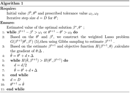
The stop condition of the algorithm is controlled by tolerance value ${\omega }_1\mathrm{,}{\omega }_2$ . In this paper we set the tolerance value equals 0.02 in the numerical simulation. Based on the discussion above, we summarise our algorithm as follows:

3.2. Theoretical Analysis

First we want to prove that the objective function (6) is guaranteed to be non-increasing at each iteration:

$H\left({\theta }^t\mathrm{,}{\beta }^t\right)\ge H\left({\theta }^t\mathrm{,}{\beta }^{t+1}\right)\ge H\left({\theta }^{t+1}\mathrm{,}{\beta }^{t+1}\right)$ (14)

Since we obtain ${\theta }^{t+1}$ by the gradient descent method, it is obvious that $H\left({\theta }^t\mathrm{,}{\beta }^{t+1}\right)\le H\left({\theta }^{t+1}\mathrm{,}{\beta }^{t+1}\right)$ .

On the other hand, we prove $H\left({\theta }^t\mathrm{,}{\beta }^t\right)\ge H\left({\theta }^t\mathrm{,}{\beta }^{t+1}\right)$ using the next lemma which has been introduced by [12] :

LEMMA: Given that the adjust parameter $\phi >0$ , then we have the following inequality:

$\arctan \left(\phi \left|{\beta }_i^t\right|\right)-\arctan \left(\phi \left|{\beta }_i^{t+1}\right|\right)\ge \frac{\phi }{1+{\phi }^2{\left|{\beta }_i^t\right|}^2}\left(\left|{\beta }_i^t\right|-\left|{\beta }_i^{t+1}\right|\right)$ (15)

proof:

We first denote $f\left(x\right)=\arctan \left(x\right)$ and let $x\ge 0$ , then by the mean value theorem we have: $f\left(x_1\right)-f\left(x_2\right)=f^{\prime }\left(\zeta \right)\left(x_1-x_2\right)$ , where $\zeta$ between $x_1$ and $x_2$ .

Since $f\left(x\right)$ is an increasing function and $f^{\prime }\left(x\right)$ is a decreasing function, the following inequality: $f\left(x_1\right)-f\left(x_2\right)\ge f^{\prime }\left(x_1\right)\left(x_1-x_2\right)$ is always holds for any non-negative value $x_1$ and $x_2$ . If we let $x_1=\phi \left|{\beta }_i^t\right|$ and $x_2=\phi \left|{\beta }_i^{t+1}\right|$ , the inequality (15) would be certainly proved.

Next we consider the following equality:

$\begin{array}{l}H\left({\theta }^t,{\beta }^t\right)-H\left({\theta }^t,{\beta }^{t+1}\right)\\ ={\Vert Y-X\left({\theta }^t\right){\beta }^t\Vert }_2^2+\lambda {\displaystyle \underset{i=1}{\overset{k}{\sum }}}\arctan \left(\phi \left|{\beta }_i^t\right|\right)-{\Vert Y-X\left({\theta }^t\right){\beta }^{t+1}\Vert }_2^2\\ -\lambda {\displaystyle \underset{i=1}{\overset{k}{\sum }}}\arctan \left(\phi \left|{\beta }_i^{t+1}\right|\right)\\ ={\Vert X\left({\theta }^t\right){\beta }^t\Vert }_2^2+{\Vert X\left({\theta }^t\right){\beta }^{t+1}\Vert }_2^2-2{\left(Y-X\left({\theta }^t\right){\beta }^t\right)}^{\prime }X\left({\theta }^t\right){\beta }^t\\ +2{\left(Y-X\left({\theta }^t\right){\beta }^{t+1}\right)}^{\prime }X\left({\theta }^t\right){\beta }^{t+1}+\lambda {\displaystyle \underset{i=1}{\overset{k}{\sum }}}\left(\arctan \left(\phi \left|{\beta }_i^t\right|\right)-\arctan \left(\phi \left|{\beta }_i^{t+1}\right|\right)\right)\end{array}$

$\begin{array}{l}={\Vert X\left({\theta }^t\right){\beta }^{t+1}-X\left({\theta }^t\right){\beta }^t\Vert }_2^2+2{\left(X\left({\theta }^t\right){\beta }^{t+1}-X\left({\theta }^t\right){\beta }^t\right)}^{\prime }X\left({\theta }^t\right){\beta }^t\\ -2{\left(Y-X\left({\theta }^t\right){\beta }^t\right)}^{\prime }X\left({\theta }^t\right){\beta }^t+2{\left(Y-X\left({\theta }^t\right){\beta }^{t+1}\right)}^{\prime }X\left({\theta }^t\right){\beta }^{t+1}\\ +\lambda {\displaystyle \underset{i=1}{\overset{k}{\sum }}}\left(\arctan \left(\phi \left|{\beta }_i^t\right|\right)-\arctan \left(\phi \left|{\beta }_i^{t+1}\right|\right)\right)\\ ={\Vert X\left({\theta }^t\right){\beta }^{t+1}-X\left({\theta }^t\right){\beta }^t\Vert }_2^2+2\left[\left(Y-X\left({\theta }^t\right){\beta }^{t+1}\right)X\left({\theta }^t\right)\left({\beta }^{t+1}-{\beta }^t\right)\right]\\ +\lambda {\displaystyle \underset{i=1}{\overset{k}{\sum }}}\left(\arctan \left(\phi \left|{\beta }_i^t\right|\right)-\arctan \left(\phi \left|{\beta }_i^{t+1}\right|\right)\right)\end{array}$ (16)

using the lemma above we can yields:

$\begin{array}{l}H\left({\theta }^t,{\beta }^t\right)-H\left({\theta }^t,{\beta }^{t+1}\right)\\ \ge {\Vert X\left({\theta }^t\right){\beta }^{t+1}-X\left({\theta }^t\right){\beta }^t\Vert }_2^2+2\left[\left(Y-X\left({\theta }^t\right){\beta }^{t+1}\right)X\left({\theta }^t\right)\left({\beta }^{t+1}-{\beta }^t\right)\right]\\ +\lambda {\displaystyle \underset{i=1}{\overset{k}{\sum }}}\frac{\phi }{1+{\phi }^2{\left|{\beta }_i^t\right|}^2}\left(\left|{\beta }_i^t\right|-\left|{\beta }_i^{t+1}\right|\right)\end{array}$ (17)

where ${\beta }_i^{t+1}$ is the optimal solution of problem (10), which satisfied:

$\frac{\partial G\left({\beta }^{t+1}|{\theta }^t,{\beta }^t\right)}{\partial {\beta }_i^{t+1}}=0$ (18)

Substituting (18) to (17), we show that we have the inequality:

$H\left({\theta }^t\mathrm{,}{\beta }^t\right)\le H\left({\theta }^t\mathrm{,}{\beta }^{t+1}\right)$ (19)

in different situations:

When: ${\beta }_i^{t+1}\ge 0$ :

$2\left[{\left(Y-X\left({\theta }^t\right){\beta }^{t+1}\right)}^{\prime }X\left({\theta }^t\right)\left({\beta }^{t+1}-{\beta }^t\right)\right]=\lambda {\displaystyle \underset{i=1}{\overset{k}{\sum }}}\frac{\phi }{1+{\phi }^2{\left|{\beta }_i^t\right|}^2}\left({\beta }_i^{t+1}-{\beta }_i^t\right)$ (20)

then:

$\begin{array}{l}H\left({\theta }^t\mathrm{,}{\beta }^t\right)-H\left({\theta }^t\mathrm{,}{\beta }^{t+1}\right)\\ \ge {\Vert X\left({\theta }^t\right){\beta }^{t+1}-X\left({\theta }^t\right){\beta }^t\Vert }_2^2+\lambda {\displaystyle \underset{i=1}{\overset{k}{\sum }}}\frac{\phi }{1+{\phi }^2{\left|{\beta }_i^t\right|}^2}\left({\beta }_i^{t+1}-{\beta }_i^t+\left|{\beta }_i^t\right|-\left|{\beta }_i^{t+1}\right|\right)\end{array}$ (21)

By the fact that ${\beta }_i^{t+1}-{\beta }_i^t+\left|{\beta }_i^t\right|-\left|{\beta }_i^{t+1}\right|\ge 0$ on the condition of ${\beta }_i^{t+1}>0$ , the inequality (19) has proved to be correct.

When: ${\beta }_i^{t+1}\le 0$ :

$2\left[{\left(Y-X\left({\theta }^t\right){\beta }^{t+1}\right)}^{\prime }X\left({\theta }^t\right)\left({\beta }^{t+1}-{\beta }^t\right)\right]=-\lambda {\displaystyle \underset{i=1}{\overset{k}{\sum }}}\frac{\phi }{1+{\phi }^2{\left|{\beta }_i^t\right|}^2}\left({\beta }_i^{t+1}-{\beta }_i^t\right)$ (22)

then:

$\begin{array}{l}H\left({\theta }^t\mathrm{,}{\beta }^t\right)-H\left({\theta }^t\mathrm{,}{\beta }^{t+1}\right)\\ \ge {\Vert X\left({\theta }^t\right){\beta }^{t+1}-X\left({\theta }^t\right){\beta }^t\Vert }_2^2+\lambda {\displaystyle \underset{i=1}{\overset{k}{\sum }}}\frac{\phi }{1+{\phi }^2{\left|{\beta }_i^t\right|}^2}\left({\beta }_i^t-{\beta }_i^{t+1}+\left|{\beta }_i^t\right|-\left|{\beta }_i^{t+1}\right|\right)\end{array}$ (23)

By the fact that ${\beta }_i^t-{\beta }_i^{t+1}+\left|{\beta }_i^t\right|-\left|{\beta }_i^{t+1}\right|\ge 0$ on the condition of ${\beta }_i^{t+1}<0$ , the inequality (19) has proved to be correct.

When: ${\beta }_i^{t+1}=0$ :

The set of sub-gradient at ${\beta }_i^{t+1}$ (which is $\left[\hat{a}\mathrm{,}\hat{b}\right]$ ) should contains 0 when ${\beta }_i^{t+1}$ is the critical point, thus we have the following inequality:

$-2{\left(X^{\prime }\left(\theta \right)Y\right)}_i-\frac{\phi \lambda }{1+{\phi }^2{\left|{\beta }_i^t\right|}^2}\le 0,-2{\left(X^{\prime }\left(\theta \right)Y\right)}_i+\frac{\phi \lambda }{1+{\phi }^2{\left|{\beta }_i^t\right|}^2}\ge 0$ (24)

Consider the inequality we want to prove, we can easily formulate:

$\begin{array}{l}H\left({\theta }^t\mathrm{,}{\beta }^t\right)-H\left({\theta }^t\mathrm{,}{\beta }^{t+1}\right)\\ \ge {\Vert X\left({\theta }^t\right){\beta }^t\Vert }_2^2+{\displaystyle \underset{i\mathrm{<mo>\; =\; </mo>\; 1}}{\overset{k}{\sum }}}\frac{\lambda \phi }{1+{\phi }^2{\left|{\beta }_i^t\right|}^2}\left(\left|{\beta }_i^t\right|-{\beta }_i^t\right)\ge 0\end{array}$ (25)

The discussion above proves that we can ensure that the function value keeps non-increasing at each iteration. In addition we want to illustrate that ${\beta }^{t+1}$ convergence to ${\beta }^{\mathrm{<mo>\; *\; </mo>}}$ and ${\theta }^{t+1}$ convergence to ${\theta }^{\mathrm{<mo>\; *\; </mo>}}$ on the limit situation ${\beta }^t\to {\beta }^{\mathrm{<mo>\; *\; </mo>}}$ and ${\theta }^t\to {\theta }^{\mathrm{<mo>\; *\; </mo>}}$ .

As ${\beta }^{t+1}$ is the optimal solution of (10), we define: ${\hat{\beta }}^{t+1}={\lim }_{\beta \to {\beta }^{*},\theta \to {\theta }^{*}}{\beta }^{t+1}$ .

Consider the first-order condition of ${\beta }^{t+1}$ which satisfied:

$\underset{\beta \to {\beta }^{*},\theta \to {\theta }^{*}}{\lim }\frac{\partial G\left(\beta |{\beta }^t,{\theta }^t\right)}{\partial {\beta }_i^{t+1}}=0$ (26)

On the other hand we have the following conclusion in the situation of ${\beta }^{\mathrm{<mo>\; *\; </mo>}}\ne 0$ :

$\frac{\partial H\left(\beta ,\theta \right)}{\partial {\beta }_i^{*}}=0$ (27)

Compare the above two equalities we can conclude that ${\hat{\beta }}^{t+1}={\beta }^{*}$ .

As for the situation when ${\beta }^{t+1}=0$ , consider the inequality from (18):

$\begin{array}{l}-2{\left(X^{\prime }\left(\theta \right)Y\right)}_i-\frac{\phi \lambda }{1+{\phi }^2{\left|{\beta }_i^{*}\right|}^2}\le 0\\ -2{\left(X^{\prime }\left(\theta \right)Y\right)}_i+\frac{\phi \lambda }{1+{\phi }^2{\left|{\beta }_i^{*}\right|}^2}\ge 0\end{array}$ (28)

Since $\frac{\phi \lambda }{1+{\phi }^2{\left|{\beta }_i^{*}\right|}^2}\le \phi \lambda$ , we can easily conclude:

$\begin{array}{l}-2{\left(X^{\prime }\left(\theta \right)Y\right)}_i-\phi \lambda \le 0\\ -2{\left(X^{\prime }\left(\theta \right)Y\right)}_i+\phi \lambda \ge 0\end{array}$ (29)

After the discussion before we can summarize that ${\hat{\beta }}^{t+1}$ always satisfied the first-order condition (7) when ${\beta }^t\to {\beta }^{\mathrm{<mo>\; *\; </mo>}}$ and ${\theta }^t\to {\theta }^{\mathrm{<mo>\; *\; </mo>}}$ . Thus we demonstrate the limit of: ${\beta }^{t+1}\to {\beta }^{\mathrm{<mo>\; *\; </mo>}}$ . When ${\theta }^t\to {\theta }^{\mathrm{<mo>\; *\; </mo>}}$ , consider the gradient of ${\theta }^t$ :

$\underset{\theta \to {\theta }^{*}}{\lim }\frac{\partial H\left({\beta }^{t+1}\mathrm{,}\theta \right)}{\partial {\theta }^t}=0$ (30)

Thus the value of ${\theta }^{t+1}$ remains ${\theta }^{\mathrm{<mo>\; *\; </mo>}}$ .

3.3. The Bayesian Lasso

In this article we use the ideal of Bayesian lasso to estimate the optimal solution of problem (10).

Assuming that the prior distribution of the parameter $\beta$ follows the Laplace distribution:

$f\left({\beta }_i\right)=\frac{\lambda }{4{\sigma }^2}\exp \left(-\frac{\lambda }{2{\sigma }^2}\left|{\beta }_i\right|\right)$ (31)

Combined with the likelihood function we can get the posterior probability:

$f\left(\beta |Y\right)\propto \exp \left(-\frac{1}{2{\sigma }^2}{\Vert Y-X\beta \Vert }_2^2-{\displaystyle \underset{i=1}{\overset{k}{\sum }}}\frac{\lambda }{2{\sigma }^2}\left|{\beta }_i\right|\right)$ (32)

Solving problem (10) is equivalent to solving the maximal probability of posterior probability, which we can obtain from Gibbs sampling [13] .

As Laplace distribution is difficult to directly derive intuitive full condition posterior distribution, the following integral (33) provides an effective solution:

$\frac{a}{2}\exp \left(-a\left|z\right|\right)={\displaystyle {\int }_0^{\infty }}\frac{1}{{\left(2\text{π}v\right)}^{1/2}}\exp \left(\frac{-z^2}{2v}\right)\times \frac{a^2}{2}\exp \left(\frac{-a^{2}v}{2}\right)\text{d}v$ (33)

Using the above integral we can rewritten the Laplace prior distribution

${\beta }_i~\frac{a}{2}\exp \left(-a\left|z\right|\right)$ by introducing the intermediate parameter v:

$\begin{array}{l}f\left({\beta }_i\right)~N\left(0,v_i\right)\\ f\left(v_i\right)~\exp \left(\frac{a^2}{2}\right)\end{array}$ (34)

In problem (32) we let $a=\frac{\lambda }{2{\sigma }^2}$ .

Then we can motivate the following hierarchical Bayesian lasso model:

$\begin{array}{l}L\left(Y|\beta ,X\right)~N\left(X\beta ,{\sigma }^{2}I\right)\\ f\left(\beta |V\right)~N\left(0,D_v\right)\\ f\left(v_i\right)~\exp \left(\frac{{\lambda }^2}{8{\sigma }^4}\right)\end{array}$ (35)

where $V=\left[v_1,\cdots ,v_k\right]$ corresponds to $\beta =\left[{\beta }_1,\cdots ,{\beta }_k\right]$ and $D_v=diag\left[v_1,\cdots ,v_k\right]$ .

For Bayesian inference, the full condition distribution of $\beta$ and v is:

$\begin{array}{l}f\left(\beta \mathrm{<mo>\; |\; </mo>}V\mathrm{,}Y\right)~N\left(A^{-1}{X}^{t}Y\mathrm{,}{\sigma }^2{A}^{-1}\right)\\ f\left(\frac{1}{v_i}\mathrm{<mo>\; |\; </mo>}{\beta }_i\mathrm{,}Y\right)~I-G\left(a^{\mathrm{<mo>\; *\; </mo>}}\mathrm{,}{b}^{\mathrm{<mo>\; *\; </mo>}}\right)\end{array}$ (36)

where $A^{-1}=X^{t}X+D_v$ , the distribution $I-G\left(a^{\mathrm{<mo>\; *\; </mo>}}\mathrm{,}{b}^{\mathrm{<mo>\; *\; </mo>}}\right)$ represent inverse Gaussian

distribution with $a^{*}=\frac{{\lambda }^{*}}{{\beta }_i}$ , $b^{*}={\left({\lambda }^{*}\right)}^2$ and ${\lambda }^{*}=\frac{\lambda }{2{\sigma }^2}$ . The density of inverse

Gaussian as follows:

$f\left(x,a^{*},b^{*}\right)={\left(\frac{\lambda }{2\text{π}{x}^3}\right)}^{\frac{1}{2}}\exp \left(-\frac{-b^{*}{\left(x-a^{*}\right)}^2}{2{\left(a^{*}\right)}^{2}x}\right)$ (37)

By repeated sampling, we will form a Markov chain contains a series of point:

$\left({\beta }_1^t\mathrm{,}{v}_1\right)\mathrm{,}\left({\beta }_2^t\mathrm{,}{v}_2\right)\mathrm{,}\cdots \mathrm{,}\left({\beta }_m^t\mathrm{,}{v}_m\right)$ .

Since each iteration will lead to a Markov chain, we will get a long sample of $\beta$ through the whole algorithm:

$\begin{array}{l}{\beta }_1^1,\cdots ,{\beta }_l^1,\cdots ,{\beta }_k^1\to {\beta }^2,{\theta }^2\\ {\beta }_1^2,\cdots ,{\beta }_l^2,\cdots ,{\beta }_k^2\to {\beta }^3,{\theta }^3\\ ⋮\\ {\beta }_1^T,\cdots ,{\beta }_l^T,\cdots ,{\beta }_k^T\to {\beta }^{*},{\theta }^{*}\end{array}$ (38)

And we have demonstrated that $H\left({\theta }^t,{\beta }^t\right)\ge H\left({\theta }^t,{\beta }^{t+1}\right)\ge \cdots \ge H\left({\theta }^{*},{\beta }^{*}\right)$ in the above. The simulation results are shown in the next section.

4. Simulation Results

In this section, we carry out a series of experiments to illustrate the performance of our proposed $l_1$ iterative reweighted algorithm (denoted to as l1-IR). In our simulations, we compare our proposed algorithm with other existing state-of-the-art methods, including the sparse Bayesian learning with dictionary refinement algorithm (denoted as DicRefCS) [7] , the sparse Bayesian learning with dictionary estimation (denoted as SBL-DE) [8] , and especially the super-resolution iterative reweighted algorithm (denoted as SR-IR) [11] .

In order to control the noise level at some of the experiments, we first give the definition of observation quality by the peak-signal-to-noise ratio (PSNR):

$PSNR\equiv 10{\log }_{10}\left(1/{\sigma }^2\right)$ (39)

where ${\sigma }^2$ represents the variance of noise. We calculate the signal-to-noise ratio (PSNR) to complete the recovery effect comparison:

$RSNR=20{\log }_{10}\left(\frac{{\Vert {\beta }^{*}\Vert }_2^2}{{\Vert {\beta }^{*}-\hat{\beta }\Vert }_2^2}\right)$ (40)

where ${\beta }^{\mathrm{<mo>\; *\; </mo>}}$ represents the original sparse signal and $\hat{\beta }$ represents the signal recovered by the algorithm. Parameters $\lambda$ and $\phi$ have the same effect as regularization parameters, we choose $\phi =1$ and select optimal parameters $\lambda$ by cross validation.

In the following, we examine the behaviour of respective algorithms under different scenarios. First we control the noise level $PSNR=20$ , which means ${\sigma }^2=0.01$ . Figure 1 shows the changes in PSNR of the various algorithms with the change of sparseness S (the sparseness S represents the number of non-zero values in original sparse signal). We keep $K=64$ and the sparseness S values range from 1 to 10. We set the number of measurements $N=20$ in order to control the variables. Each data point is averaged by repeated tests.

Figure 1 indicates that the performance of the $l_1$ iterative reweighted algorithm is better than other state-of-the-art methods. With a low sampling number ( $N=20$ ), the performances of the DicRefCS and SBL-DE algorithms deteriorated quickly and failed when the sparseness S was higher than 5. On the other hand, our proposed algorithm still performed well, even when the sparseness S reached 8. It is worth mentioning that the SR-IR algorithm also performed better than the other two Bayesian algorithms but not as well as the L1-IR algorithm. The reasons are that the $l_1$ norm is sparser than the $l_2$ norm and we chose a better weight function.

Next, we illustrate the influence of the sample size N on the recovery effect using another set of experiments. We keep $K=64$ , the sparseness $S=3$ and the PSNR maintains at 20. We change the number of measurements N from 6 to 32. For each N, Figure 2 shows the performance of respective algorithms.

It can be observed from Figure 2 that, with the increase in N, the recovery performance of the respective algorithms is increased to a relatively high level but our proposed algorithm outperforms the other methods for a small number

Figure 1. RSNR in different S while K = 64, n = 20, PSNR = 20.

of measurements. This means that our method performs better for the recovery of sparse signals when the number of samples is limited.

Our last experiment tested the recovery performance of respective algorithm under different noise level PSNR. According to the definition of PSNR, we set the variance of noise from 0.01 to 1, which makes the PSNR changed from 20 to 0. At this experiment use signals of length $K=64$ contains $S=3$ complex sinusoids and set the number of measurements $N=24$ . We take 20 points evenly between 0 and 20 and record the performance of respective algorithm in each point. Each data point is averaged by repeated tests.

Relatively speaking, the L1-IR algorithm and the SR-IR algorithm were more stable than the other algorithms as the noise level increased. Figure 3 indicates that the PSNR of all algorithms deteriorated quickly when the noise was very strong. In the case of relatively strong noise, some trials lead to failure results and the failure rate increases with an increasing noise level. Here, a trial was considered successful if the PSNR was higher than 15 dB. Table 1 shows the success rate of the algorithms for different levels of PSNR (at each level, we repeated 20 trials) in the last experiment. The success rate of DicRefCS and SBL-DE is obviously less than that of l1-IR and SR-IR when $sigm{a}^2$ is large than 0.2.

The validity, superiority, and stability of the l1-IR algorithm are illustrated by these experiments, indicating that the algorithm is worth applying in some practical cases.

5. Conclusion

In this paper, we treated the real dictionary parameters as unknown variables, and studied the line spectral estimation problem with unknown dictionary parameters. Based on the ideal of Bayesian lasso and the analysis of the first-order

Figure 2. RSNR in different n while K = 64, S = 3, PSNR = 20.

Figure 3. RSNR in different noise level while K = 64, S = 3, n = 20.

Table 1. Successful rate of different algorithms.

condition of the optimal solution, we proposed an iterative reweighted $l_1$ penalty regression algorithm. We proved that in each step of the iterative process, the function value is continuously reduced until the approximate solution of the real sparse vector is obtained. The numerical results in Section 4 illustrated that the performance of our algorithm is better than other state-of-the-art algorithms in some cases. The disadvantage is that our method is more time-consuming, partly because in each sampling step it is necessary to ensure convergence, resulting in a sampling length that cannot be effectively reduced. Future studies will focus on this problem.

Conflicts of Interest

The authors declare no conflicts of interest.

References

[1]	Chi, Y.J., Scharf, L.L., Pezeshki, A. and Calderbank, A.R. (2011) Sensitivity to Basis Mismatch in Compressed Sensing. IEEE Transactions on Signal Process, 59, 2182-2195. https://doi.org/10.1109/TSP.2011.2112650
[2]	Tan, Z., Yang, P. and Nehorai, A. (2014) Joint Sparse Recovery Method for Compressed Sensing with Structured Dictionary Mismatches. IEEE Transactions on Signal Process, 62, 4997-5008. https://doi.org/10.1109/TSP.2014.2343940
[3]	Fannjiang, A. and Liao, W. (2014) Coherence Pattern-Guided Compressive Sensing with Unresolved Grids. SIAM Journal on Imaging Sciences, 5, 179-202. https://doi.org/10.1137/110838509
[4]	Duarte, M.F. and Baraniuk, R.G. (2013) Spectral Compressive Sensing. Applied and Computational Harmonic Analysis, 35, 111-129. https://doi.org/10.1016/j.acha.2012.08.003
[5]	Candes, E. and Fernandez-Granda, C. (2014) Towards a Mathematical Theory of Super-Resolution. Communications on Pure and Applied Mathematics, 67, 906-956. https://doi.org/10.1002/cpa.21455
[6]	Tang, G., Bhaskar, B.N., Shah, P. and Recht, B. (2013) Compressed Sensing Off the Grid. IEEE Transactions on Information Theory, 59, 7465-7490. https://doi.org/10.1109/TIT.2013.2277451
[7]	Hansen, T.L., Badiu, M.A., Fleury, B.H. and Rao, B.D. (2014) A Sparse Bayesian Learning Algorithm with Dictionary Parameter Estimation. Sensor Array and Multichannel Signal Processing Workshop, A Coruna, 22-25 June 2014, 385-388. https://doi.org/10.1109/SAM.2014.6882422
[8]	Hu, L., Shi, Z., Zhou, J. and Fu, Q. (2012) Compressed Sensing of Complex Sinusoids: An Approach Based on Dictionary Refinement. IEEE Transactions on Signal Process, 60, 3809-3822. https://doi.org/10.1109/TSP.2012.2193392
[9]	Fang, J., Li, J., Shen, Y., Li, H. and Li, S. (2014) Super-Resolution Compressed Sensing: An Iterative Reweighted Algorithm for Joint Parameter Learning and Sparse Signal Recovery. IEEE Transactions on Signal Process, 21, 761-765. https://doi.org/10.1109/LSP.2014.2316004
[10]	Tibshirani, R. (1996) Regression Shrinkage and Selection via the Lasso. Journal of the royal Statistical Society. Series B, 58, 276-288.
[11]	Fang, J., Wang, F., Shen, Y. and Li, H. (2016) Super-Resolution Compressed Sensing for Line Spectral Estimation: An Iterative Reweighted Approach. IEEE Transactions on Signal Process, 64, 4649-4672. https://doi.org/10.1109/TSP.2016.2572041
[12]	Lai, M.J., Xu, Y. and Yin, W. (2013) Improved Iteratively Reweighted Least Squares for Unconstrained Smoothed lq Minimization Estimation. SIAM Journal on Numerical Analysis, 51, 927-957. https://doi.org/10.1137/110840364
[13]	Andrieu, C., Freitas, N. and Doucet, A. (2003) An Introduction to MCMC for Machine Learning. Machine Learning, 50, 5C43.