A Study of Stellar Model with Kramer’s Opacity by Using Runge Kutta Method with Programming C

Md. Abdullah Bin Masud, Shammi Akter Doly

Department of Computer Science & Engineering, Shanto-Mariam University of Creative Technology, Dhaka, Bangladesh.

DOI: 10.4236/ijaa.2017.73015                

Abstract

In this paper, we have made an investigation on a stellar model with Kramer’s Opacity and negligible abundance of heavy elements. We have determined the structure of a star with mass , i.e. the physical variables like pressure, density, temperature and luminosity at different interior points of the star. We have discussed about some equations of structure, mechanism of energy production in a star and energy transports in stellar interior in a star and then we have solved radiative envelope and convective core by the matching or fitting point method and Runge-Kutta method by C Programming language. In future, it will help us to know about the characteristics of new stars.

Keywords

Energy Production in Star, Hydrostatic Equilibrium of Star, Mass Conservation, Schwarzschild Method and Variable, Polytropic Core Solution, Packet Solution

1. Introduction

A star is a dense mass that generates its light and heat by nuclear reactions, specifically by the fusion of hydrogen and helium under conditions of enormous temperature and density. Stars are like our sun. The star is powered by hydrogen fusion. The fusion only takes place at core of the star where it is dense enough. The “life” of a star is the time during which it slowly burns up its hydrogen fuel, and evolves only slowly in the process. The star is in force balance between pressure and gravity. It is also in energy balance between production by fusion reactions, transport by photon radiation, and loss from the surface by the (usually) visible radiation by which can detect the star. The “birth” of a star refers to the process by which it is formed from diffuse clouds of cold gas that are present in its galaxy [1] . A cloud collapses to form a number of stars when it is disturbed so that its gravity overcomes its motion and pressure. The “death” of a star occurs when its fusion fuel, first hydrogen and then heavier nuclei, have run out. This can be very violent if the star is very massive, ending in things like a black hole and/or a supernova, perhaps leaving a neutron star behind. If the star is not very massive, like the Sun or even smaller, it ends by ejecting part of its atmosphere and then settling down to a cold, dense white dwarf. Harm & Schwarzschild (1955) have shown that the maximal possible mass of the star is $60M_{\odot }$ and minimum mass of star is $0.01M_{\odot }$ [2] . The chemical element of star is hydrogen, helium and other heavier elements [3] . If hydrogen, helium and other elements are denoted by X, Y and Z respectively, then $X+Y+Z=1$ . For the sun X = 0.73, Y = 0.25 and Z = 0.02.

2. HR Diagram

HR diagram is diagram where the absolute magnitudes and luminosities of stars are plotted against heir surface temperatures or colors. In 1905, Danish astronomer Einar Hertzsprung, and independently American astronomer Henry Norris Russell developed the technique of plotting absolute magnitude for a star versus its spectral type to look for families of stellar type. These diagrams, called the Hertzsprung-Russell or HR diagrams, plot luminosity in solar units on the Y axis and stellar temperature on the X axis [2] , as shown in Figure 1.

3. Energy Production in Stars

A normal main sequence star derives energy from its nuclear source. Enormous amount of energy are continually radiated at a steady rate over long spars of time; for example the sun radiates approximately 10⁴¹ ergs per year. Those thermonuclear reactions do produce energy. That a star can derive energy from thermonuclear reaction is understood from the following example $\text{4}{}_1\text{H}{}^{\text{1}}={}_2\text{H}{\text{e}}^{\text{4}}$ $+\text{2}{\beta }^{+}+\text{2}\nu +\gamma$ [4] [5] . That means four hydrogen atoms combine to give one helium atom with the production of two positrons (b⁺), two neutrinos (ν) and radiation (γ). Energy production mainly in two ways: 1) Proton-Proton chain (PP chain); 2) Carbon-Nitrogen chain (CN chain).

Figure 1. HR diagram.

4. Hydrostatic Equilibrium of Star

Consider a cylinder of mass dm located at a distance r from centre of the star with height dr and surface area A at the top and bottom. Also denote $F_{p.t}$ and $F_{p.b}$ to be the pressure forces at the top and bottom of the cylinder respectively

If F_g < 0 is the gravitational forces on the cylinder then from Newton’s second law we have

$\text{d}m\frac{{\text{d}}^{2}r}{\text{d}{t}^2}=F_g+F_{p.t}+F_{p.b}$ (1)

Defining the change in pressure force dF_p across the cylinder by $F_{p.t}=-\left(F_{p.b}+\text{d}{F}_p\right)$

Then gives

$\text{d}m\frac{{\text{d}}^{2}r}{\text{d}{t}^2}=F_g-\text{d}{F}_p$ (2)

The gravitational force on the small mass dm is given by

$F_g=-G\frac{M\left(r\right)\text{d}m}{r^2}$ (3)

From the definition of pressure as the force per unit area we have

$P=\frac{F}{A}\Rightarrow \text{d}{F}_p=A\text{d}P$ (4)

Putting (3) and (4) in (2)

$\text{d}m\frac{{\text{d}}^{2}r}{\text{d}{t}^2}=-G\frac{M\left(r\right)\text{d}m}{r^2}-A\text{d}P$ (5)

Assuming the density of the cylinder is r, then its mass is $\text{d}m=rA\text{d}r$ , now (5) becomes

$\rho A\text{d}r\frac{{\text{d}}^{2}r}{\text{d}{t}^2}=-G\frac{M\left(r\right)\rho A\text{d}r}{r^2}-A\text{d}P$

Dividing by volume of the cylinder gives

$\rho \frac{{\text{d}}^{2}r}{\text{d}{t}^2}=-G\frac{M\left(r\right)\rho }{r^2}-\frac{\text{d}P}{\text{d}r}$

Assuming the star is static the acceleration term will be zero which then leads to

$\frac{\text{d}P}{\text{d}r}=-G\frac{M\left(r\right)\rho }{r^2}=-\rho g$ (6)

where $g=G\frac{M\left(r\right)}{r^2}$ .

This is the condition of hydrostatic equilibrium.

5. Mass Conservation

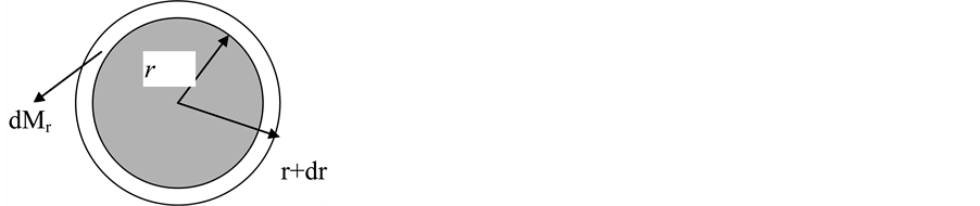
Consider a spherically symmetric shell of mass dM_r with thickness dr and r is the distance from the centre of the star. The local density is of the shell is r. The shell’s mass is then given by $\delta M=\delta V\rho \left(r\right)$ .

Since $\delta V=4\text{π}{r}^2\delta r$ . Then we have $\delta M=4\text{π}{r}^2\delta r\rho \left(r\right)$

$\Rightarrow \frac{\text{d}M\left(r\right)}{\text{d}r}=4\text{π}{r}^2\rho \left(r\right).$ (7)

In the limit where $\delta r\to 0$ , which is the mass conservation equation.

6. Energy Conservation

Consider a spherical symmetric star in which energy transport is radial in which time variations are very important. Let L_r is the rate of energy flow a across of sphere of radius r and L_r+dr for radius r + dr

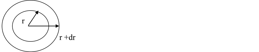
Now, the volume of the shell = $4\text{π}{r}^2\text{d}r$

If r is the density, then mass of the shell = $4\text{π}{r}^2\rho \text{d}r$ .

The energy released in the shell can be written as $4\text{π}{r}^2\rho \text{d}r\epsilon$ , where e is defined as the energy released per unit mass per unit time. The conservation of energy leads that

$L_{r+\text{d}r}-L_r=\text{4π}{r}^2\rho \epsilon \text{d}r$

$\Rightarrow \frac{\text{d}L}{\text{d}r}\cdot \text{d}r=\text{4π}{r}^2\rho \epsilon \text{d}r$

$\therefore \frac{\text{d}L}{\text{d}r}=\text{4π}{r}^2\rho \epsilon$ (8)

This is the equation of energy conservation.

7. Energy Transport in Stellar Interior

Energy transport in stellar interiors occurs by three mechanisms, i.e. radiation, convection and conduction [6] [7] .

7.1. Radiation

Photons carry energy but constantly interact with electrons and ions. Each interaction causes the photon, on average, to lose energy to the plasma ⇒ increase in gas temperature.

7.2. Convection

Energy is carried by macroscopic mass motion (rising gas) though there is no net mass flux. If the density of an element of gas is less than that of its surroundings, it rises ⇒ Schwarzschild criterion for convection.

7.3. Conduction

Energy is carried by mobile electrons, which collide with ions and other electrons, but still make progress through the star. The diffusive nature of this process makes it describable in a way similar to radiative transport.

7.4. Radiative Energy Transport

If the condition of the occurrence of convection is failed then radiative transfer occurs. The energy carried by radiation per square meter per second i.e. flux F_rad can be expressed in term of the temperature gradient and a coefficient of radiative conductively l_rad as follows

$F_{rad}=-{\lambda }_{rad}\frac{\text{d}T}{\text{d}r}$ (9)

where -ve sign indicates that heat flows down the temperature gradient.

Assuming all energy is transported by radiation. We will now drop the suffix rad,

$\therefore F=-\lambda \frac{\text{d}T}{\text{d}r}$ (10)

Astronomers prefer to work with an inverse of the conductivity known as opacity which opacity k defined as

$\kappa =\frac{4ac{T}^3}{3\rho \lambda }$ (11)

where a is the radiation density constant, c is the speed of light.

From (11) we have

$\lambda =\frac{4ac{T}^3}{3\rho \kappa }$ (12)

Putting (12) in (10) we have

$F=-\frac{4ac{T}^3}{3\kappa \rho }\frac{\text{d}T}{\text{d}r}$ (13)

We know flux and luminosity equation is

$L=4\text{π}{r}^{2}F$ (14)

$\Rightarrow L=-\frac{16ac\text{π}{r}^2{T}^3}{3\kappa \rho }\frac{\text{d}T}{\text{d}r}$ [from (13)]

$\Rightarrow \frac{\text{d}T}{\text{d}r}=-\frac{3\kappa \rho L}{16\text{π}ac{r}^2{T}^3}$ (15)

This equation is known as the equation of radiative transfer.

7.5. Convective Energy Transport

Let ${\rho }_1^{*}$ and $P_1^{*}$ be the density and pressure inside the blob in its original position, the corresponding quantities outside being r₁ and P₁. In its displaced position, let ${\rho }_2^{*}$ and $P_2^{*}$ be the density and pressure inside the blob white corresponding quantities outside be r₂ and P₂.

Before the perturbation, ${\rho }_1^{*}={\rho }_1$ and $P_1^{*}=P_1$

After the perturbation

${\rho }_2^{*}={\rho }_1^{*}{\left(\frac{P_2^{*}}{P_1^{*}}\right)}^{1/\gamma }\text{and}{P}_2^{*}=P_2$

where $\gamma$ is the ratio of specific that $\frac{C_p}{C_v}$ and has the value 5/3 for highly ionized gas. The layer may be stable if ${\rho }_2^{*}>{\rho }_2$ . Therefore mass motion will occur if ${\rho }_2^{*}<{\rho }_2$ . Now we have from the above equations ${\rho }_2^{*}={\rho }_1{\left(\frac{P_2}{P_1}\right)}^{1/\gamma }$

The equilibrium is stable if ${\rho }_1{\left(\frac{P_2}{P_1}\right)}^{1/\gamma }>{\rho }_2$

And the equilibrium is unstable if ${\rho }_1{\left(\frac{P_2}{P_1}\right)}^{1/\gamma }<{\rho }_2$

Let $P_1=P\left(r\right)$ and ${\rho }_1=\rho \left(r\right)$ , $P_2=P\left(r+\text{d}r\right)$ and ${\rho }_2=\rho \left(r+\text{d}r\right)$

From stable condition we have ${\left(\frac{P_2}{P_1}\right)}^{1/\gamma }>\frac{{\rho }_2}{{\rho }_1}$

From unstable condition we have ${\left(\frac{P_2}{P_1}\right)}^{1/\gamma }<\frac{{\rho }_2}{{\rho }_1}$

which implies ${\left(\frac{P\left(r+\text{d}r\right)}{P\left(r\right)}\right)}^{1/\gamma }>\text{or}<\frac{\rho \left(r+\text{d}r\right)}{\rho \left(r\right)}$

Or ${\left(1+\frac{1}{P}\frac{\text{d}P}{\text{d}r}\text{d}r\right)}^{1/\gamma }>\text{or}<\left(1+\frac{1}{\rho }\frac{\text{d}\rho }{\text{d}r}\text{d}r\right)$

Expanding left side of the above inequalities in Taylor series and neglecting higher order terms we have

$\left(1+\frac{1}{\lambda P}\frac{\text{d}P}{\text{d}r}\text{d}r\right)>\text{or}<\left(1+\frac{1}{\rho }\frac{\text{d}\rho }{\text{d}r}\text{d}r\right)$

$\Rightarrow \frac{1}{\gamma P}\frac{\text{d}P}{\text{d}r}>\text{or}<\frac{1}{\rho }\frac{\text{d}\rho }{\text{d}r}$

We know $P=\frac{K}{\mu H}\rho T$

Taking log and differentiating we have

$\frac{1}{P}\frac{\text{d}P}{\text{d}r}=\frac{1}{\rho }\frac{\text{d}\rho }{\text{d}r}+\frac{1}{T}\frac{\text{d}T}{\text{d}r}$

For stability condition we have

$\frac{1}{\gamma P}\frac{\text{d}P}{\text{d}r}>\frac{1}{P}\frac{\text{d}P}{\text{d}r}-\frac{1}{T}\frac{\text{d}T}{\text{d}r}$

$\Rightarrow -\left(1-\frac{1}{\gamma }\right)\frac{\text{d}P}{\text{d}r}>-\frac{P}{T}\frac{\text{d}T}{\text{d}r}$

Therefore mass motion will occur when

$-\left(1-\frac{1}{\gamma }\right)\frac{\text{d}P}{\text{d}r}<-\frac{P}{T}\frac{\text{d}T}{\text{d}r}$

Schwarzschild (1958) has shown that the temperature gradient for the convection is well represented by

$\frac{\text{d}T}{\text{d}r}=\left(1-\frac{1}{\gamma }\right)\frac{T}{P}\frac{\text{d}P}{\text{d}T}$ (16)

which is known as convective energy equation [2] .

8. Schwarzschild Method and Variable

When one is searching for the numerical solution to a physical problem, it is convenient to re-express the problem in terms of a set of dimensionless variables whose range is known and conveniently limited. This is exactly what the Schwarzschild variables accomplish. Define the following set of dimensionless variables [2]

$x=\frac{r}{R}$ (17)

$q=\frac{M\left(r\right)}{M}$ (18)

$l=\frac{L\left(r\right)}{L}$ (19)

$p=P\left(r\right)\frac{4\text{π}{R}^4}{G{M}^2}$ (20)

$t=T\left(r\right)\frac{R}{\mu }\frac{R}{GM}$ (21)

$\rho \left(r\right)=\frac{M}{4\text{π}{R}^3}\frac{p}{t}$ (22)

Note that the first three variables are the fractional radius, mass and luminosity, respectively and after three variables represented the pressure, temperature and density. In addition, let us assume that the opacity and energy generation rate can be approximately by

and

$\kappa ={\kappa }_0\left(\frac{\rho }{T^{3.5}}\right)$ , ${\epsilon }_{PP}={\epsilon }_0\rho X{X}_{CN}\times {\left(\frac{T}{{10}^6}\right)}^{16}$

where

${\kappa }_0=4.34\times {10}^{25}\times Z\left(1+X\right)$

Putting (17), (18), (20) and (19) in (6), we have

$\frac{\text{d}}{\text{d}\left(Rx\right)}\left(\frac{G{M}^{2}p}{4\text{π}{R}^4}\right)=-\frac{GqM}{R^2{x}^2}\frac{M}{4\text{π}{R}^3}\frac{p}{t}$

$\Rightarrow \frac{G{M}^2}{4\text{π}{R}^5}\frac{\text{d}p}{\text{d}x}=-\frac{G{M}^2}{4\text{π}{R}^5}\frac{pq}{t{x}^2}$

$\Rightarrow \frac{\text{d}p}{\text{d}x}=-\frac{pq}{t{x}^2}$ (23)

Again, putting (17), (18) and (22) in (7), we have

$\frac{\text{d}}{\text{d}\left(xR\right)}\left(qM\right)=4\text{π}{R}^2{x}^2\frac{M}{4\text{π}{R}^3}\frac{p}{t}$

$\Rightarrow \frac{M}{R}\frac{\text{d}q}{\text{d}x}=\frac{M}{R}\frac{p{x}^2}{t}$

$\Rightarrow \frac{\text{d}q}{\text{d}x}=\frac{p{x}^2}{t}$ (24)

Now putting (17), (19), (22) and (21) in (8), we have

$\frac{\text{d}}{\text{d}\left(Rx\right)}\left(lL\right)=4\text{π}{R}^2{x}^2{\epsilon }_0{\rho }^{2}X{X}_{CN}\times {\left(\frac{T}{{10}^6}\right)}^{16}$

$\begin{array}{l}\Rightarrow \frac{L}{R}\frac{\text{d}l}{\text{d}x}={\epsilon }_{0}X{X}_{CN}4\text{π}{R}^2{x}^2{\left(\frac{M}{4\text{π}{R}^3}\frac{p}{t}\right)}^2\frac{1}{{10}^{96}}\\ \times {\left(\frac{tM}{R}\right)}^{16}{\left(\mu G\right)}^{16}{\left(\frac{1}{R}\right)}^{16}\end{array}$

$\Rightarrow \frac{\text{d}l}{\text{d}x}=\frac{{\epsilon }_{0}X{X}_{CN}}{4\times {10}^{96}\text{π}}{\left(\mu G\right)}^{16}\cdot {\left(\frac{1}{R}\right)}^{16}\cdot \frac{M^{18}}{L{R}^{19}}\cdot p^2{x}^2{t}^{14}$

$\Rightarrow \frac{\text{d}l}{\text{d}x}=D{p}^2{x}^2{t}^{14}$ (25)

where $D=\frac{{\epsilon }_{0}X{X}_{CN}}{4\times {10}^{96}\text{π}}\times {\left(\mu G\right)}^{16}\times {\left(\frac{1}{R}\right)}^{16}\times \frac{M^{18}}{L{R}^{19}}$

Again putting (17), (19), (21), (22) and (23) in (15), we get

$\frac{\text{d}}{\text{d}\left(Rx\right)}\left(\frac{GMt}{R}\right)\frac{\mu }{R}=-\frac{3{\kappa }_{0}lL}{16\text{π}ac{R}^2{x}^2}\times \frac{{\rho }^2}{T^{6.5}}$

$\Rightarrow \frac{\mu }{R}GM\frac{\text{d}t}{\text{d}x}=-\frac{3{\kappa }_{0}lL}{16\text{π}ac{x}^2}\times {\left(\frac{M}{4\text{π}{R}^3}\frac{p}{t}\right)}^2\times {\left(\frac{R}{GMt}\right)}^{6.5}\times {\left(\frac{R}{\mu }\right)}^{6.5}$

$\Rightarrow \frac{\text{d}t}{\text{d}x}=-\frac{3{\kappa }_0}{256{\text{π}}^{3}ac}{\left(\frac{1}{G}\right)}^{7.5}\frac{L{R}^{0.5}}{M^{5.5}}\frac{p^{2}l}{x^2{t}^{8.5}}$

$\Rightarrow \frac{\text{d}t}{\text{d}x}=-C\frac{p^{2}l}{x^2{t}^{8.5}}$

where $C=\frac{3{\kappa }_0}{256{\text{π}}^{3}ac}{\left(\frac{1}{G}\right)}^{7.5}\frac{L{R}^{0.5}}{M^{5.5}}$

putting (17), (19) and (20) in (16) we have

$\frac{\text{d}t}{\text{d}x}=\frac{2}{5}\frac{t}{p}\frac{\text{d}p}{\text{d}x}$ (26)

Finally we have the full set equations

$\frac{\text{d}p}{\text{d}x}=-\frac{pq}{t{x}^2}$ (27)

$\frac{\text{d}q}{\text{d}x}=\frac{p{x}^2}{t}$ (28)

$\frac{\text{d}l}{\text{d}x}=D{p}^2{x}^2{t}^{14}$ (29)

$\frac{\text{d}t}{\text{d}x}=-C\frac{p^{2}l}{x^2{t}^{8.5}}$ (Radiative layer) (30)

$\frac{\text{d}t}{\text{d}x}=\frac{2}{5}\frac{t}{p}\frac{\text{d}p}{\text{d}x}$ Convective layer (31)

which are subject to the boundary conditions

$\begin{array}{c}q\left(0\right)=l\left(0\right)=0\\ \text{and}q\left(1\right)=l\left(1\right)=1\end{array}$ (32)

If the star has a convective core, then all the energy is produced in a region where the structure is essentially specified by the adiabatic gradient and so the energy conservation Equation (29) is redundant. This means that the D is unspecified and the problem will be solved by determining C alone. Such a model is known as a Cowling model.

9. Solution of the Model

Since the model star is likely to have a small convective core with a radiative envelope, in principle we have two solutions, one is the envelope and another is the core. The two solutions must match at the interface.

a) Polytropic Core Solution

b) Packet Solution

9.1. Polytropic Core Solution

Eliminating q from (27) and (28) we have

$\frac{\text{d}}{\text{d}x}\left(-\frac{t{x}^2}{p}\frac{\text{d}p}{\text{d}x}\right)=\frac{p{x}^2}{t}$

$\Rightarrow \frac{\text{d}}{\text{d}x}\left(-\frac{t{x}^2}{p}\frac{5p}{2t}\frac{\text{d}t}{\text{d}x}\right)=\frac{p{x}^2}{t}$ [from (3.3)]

$\Rightarrow \frac{5}{2}\frac{\text{d}}{\text{d}x}\left(x^2\frac{\text{d}t}{\text{d}x}\right)=-\frac{p{x}^2}{t}$ (33)

Now introducing the polytropic variables $\eta$ and $\theta$ , defined by

$p=p_c{\theta }^{5/2},t=t_c\theta ,x={\left(\frac{5}{2}\frac{t_c^2}{p_c}\right)}^{1/2}\eta$

where p_c and t_c are the central pressure and temperature in non-dimensional. Now putting the value of p, t and x in (3.4), we have

$\begin{array}{l}\frac{5}{2}{\left(\frac{2p_c}{5t_c^2}\right)}^{1/2}\frac{\text{d}}{\text{d}\eta }\left(\frac{5}{2}\frac{t_c^2}{p_c}{\eta }^2{\left(\frac{2p_c}{5t_c^2}\right)}^{1/2}{t}_c\frac{\text{d}\theta }{\text{d}\eta }\right)\\ =-\frac{5p_c{\theta }^{5/2}}{2}\frac{t_c^2}{p_c}{\eta }^2\frac{1}{t_c\theta }\end{array}$

$\Rightarrow \frac{5}{2}\frac{2p_c}{5t_c^2}\frac{t_c^3}{p_c}\frac{\text{d}}{\text{d}\eta }\left({\eta }^2\frac{\text{d}\theta }{\text{d}\eta }\right)=-{\eta }^2{t}_c{\theta }^{3/2}$

$\Rightarrow \frac{1}{{\eta }^2}\frac{\text{d}}{\text{d}\eta }\left({\eta }^2\frac{\text{d}\theta }{\text{d}\eta }\right)=-{\theta }^{3/2}$ (34)

which is the Lane-Emden equation with index $n=\frac{3}{2}$ .

The general solution of (34) is

$\begin{array}{l}\theta =1-\frac{1}{6}{\eta }^2+\frac{\frac{3}{2}}{120}{\eta }^4-\frac{\frac{3}{2}\left(8\times \frac{3}{2}-5\right)}{42\times 360}{\eta }^6+\cdots \\ \Rightarrow \theta =1-\frac{1}{6}{\eta }^2+\frac{1}{80}{\eta }^4-\frac{1}{1440}{\eta }^6+\cdots \end{array}$

For small $\eta$ this is a rapidly convergent series.

We take

$\theta =1-\frac{1}{6}{\eta }^2+\frac{1}{80}{\eta }^4$ (35)

Introducing Schwarzschild homology variables defined by [2]

$\begin{array}{c}U\equiv \frac{\text{d}\ln M\left(r\right)}{\text{d}\ln r}=\frac{r}{M\left(r\right)}\frac{\text{d}M\left(r\right)}{\text{d}r}=\frac{xR}{qM}\frac{M\text{d}q}{R\text{d}x}=\frac{x}{q}\frac{\text{d}q}{\text{d}x}\\ =-\frac{x}{\frac{t{x}^2}{p}\frac{\text{d}p}{\text{d}x}}\cdot \frac{p{x}^2}{t}=-\frac{p^{2}x}{t^2\frac{\text{d}p}{\text{d}x}}=-\frac{p^{2}x}{t^2\frac{5p}{2t}\frac{\text{d}t}{\text{d}x}}=-\frac{2}{5}\frac{px}{t}\frac{1}{\frac{\text{d}t}{\text{d}x}}\\ =-\frac{2}{5}\frac{p_c{\theta }^{5/2}}{t_c\theta }{\left(\frac{5}{2}\frac{t_c^2}{p_c}\right)}^{1/2}\eta \frac{1}{\frac{t_c}{{\left(\frac{5}{2}\frac{t_c^2}{p_c}\right)}^{1/2}}\frac{\text{d}\theta }{\text{d}\eta }}\\ =-\frac{2}{5}\frac{p_c}{t_c^2}{\theta }^{3/2}\frac{5}{2}\frac{t_c^2}{p_c}\eta \frac{1}{\frac{\text{d}\theta }{\text{d}\eta }}=-{\theta }^{3/2}\eta \frac{1}{\frac{\text{d}\theta }{\text{d}\eta }}\cong 3-\frac{3{\eta }^2}{10}+\cdots \end{array}$

$\begin{array}{c}\text{and}V\equiv -\frac{\text{d}\ln P}{\text{d}\ln r}=-\frac{r}{P}\frac{\text{d}P}{\text{d}r}=-\frac{xR}{\frac{G{M}^2}{4\text{π}{R}^4}p}\frac{G{M}^2}{4\text{π}{R}^4}\frac{\text{d}p}{R\text{d}x}\\ =-\frac{x}{p}\frac{\text{d}p}{\text{d}x}=-\frac{{\left(2.5t_c^2/p_c\right)}^{1/2}\eta }{p_c{\theta }^{5/2}}\frac{\text{d}{\theta }^{5/2}}{{\left(2.5t_c^2/p_c\right)}^{1/2}\text{d}\eta }\\ =-\frac{\eta }{{\theta }^{5/2}}\frac{\text{d}{\theta }^{5/2}}{\text{d}\eta }\cong \frac{5{\eta }^2}{6}\left(1+\frac{{\eta }^2}{60}+\cdots \right)\end{array}$

So as to good approximation

$U=3-\frac{18}{50}V$ (36)

This gives the core solution in the U-V plane.

9.2. Packet Solution

The Equation (30) contains an unknown parameter C. Our aim is to determine the correct value of C and obtain the packet solution for the value of the parameter. In order to do this we have to solve the packet solutions for different trial value of C and find which value of C the solution just matches the core solution at the interface. The packet solutions we have calculated numerically, however since the equations are singular at the surface, $p=t=0$ .

Let $\frac{1}{x}-1=\gamma \Rightarrow \text{d}x=-x^2\text{d}\gamma$

$\therefore \frac{\text{d}p}{\text{d}x}=-\frac{qp}{t{x}^2}\Rightarrow \frac{\text{d}p}{-x^2\text{d}\gamma }=-\frac{qp}{t{x}^2}\Rightarrow \frac{\text{d}p}{\text{d}\gamma }=\frac{qp}{t}\Rightarrow t\frac{\text{d}p}{\text{d}\gamma }=qp$

and $\frac{\text{d}t}{\text{d}x}=-C\frac{p^2}{t^{8.5}{x}^2}$ Math_126#

$\Rightarrow \frac{\text{d}t}{\text{d}\gamma }=C\frac{p^2}{t^{8.5}}$ Math_128#

and $\frac{\text{d}q}{\text{d}x}=\frac{p{x}^2}{t}$ Math_130##Math_131#

$\Rightarrow \frac{\text{d}q}{\text{d}\gamma }=-\frac{p}{t{\left(1+\gamma \right)}^4}$

Here the singular point is $\gamma =0$ , since x = 1 i.e. $\gamma =0$ . Now the series expansion of variables about $\gamma =0$ can be easily done. By Fuchs theorem, a convergent development of the solution in a power series about the singular point having a finite number of terms is possible.

We therefore take $t={\gamma }^u\left(a_0+a_1\gamma +\cdots +a_n{\gamma }^n\right)$

$p={\gamma }^v\left(b_0+b_1\gamma +\cdots +b_n{\gamma }^n\right)$

and $q=1+c_1\gamma +c_2{\gamma }^2+\cdots +c_n{\gamma }^n$

We have

$\begin{array}{l}{\gamma }^u\left(a_0+a_1\gamma +\cdots +a_n{\gamma }^n\right)\frac{\text{d}}{\text{d}\xi }\left\{{\gamma }^v\left(b_0+b_1\gamma +\cdots +b_n{\gamma }^n\right)\right\}\\ =\left(1+c_1\gamma +\cdots +c_n{\gamma }^n\right)\left\{{\gamma }^v\left(b_0+b_1\gamma +\cdots +b_n{\gamma }^n\right)\right\}\end{array}$

$\begin{array}{l}\Rightarrow a_0{b}_{0}v{\gamma }^{u+v-1}+\left(a_1{b}_{0}v+a_0{b}_1\right){\gamma }^{u+v}+\cdots \\ =b_0{\gamma }^v+\left(b_1+b_0{c}_1\right){\gamma }^{v+1}+\cdots \end{array}$

Since the two polynomial are equal must have $u+v-1=v$ and $u+v=v+1$ and $a_0{b}_{0}v=b_0$

$\therefore u=1\text{and}{a}_{0}v=1$

We have

$t=a_0\gamma +a_1{\gamma }^2+\cdots +a_n{\gamma }^{n+1}$

$\begin{array}{l}\therefore {\left(a_0\gamma +a_1{\gamma }^2+\cdots +a{}_n\gamma {}^{n+1}\right)}^{8.5}\frac{\text{d}}{\text{d}\gamma }\left(a_0\gamma +a_1{\gamma }^2+\cdots +a{}_n\gamma {}^{n+1}\right)\\ =C{\left(b_0{\gamma }^v+b_1{\gamma }^{v+1}+\cdots +b_n{\gamma }^{v+n}\right)}^2\end{array}$

$\begin{array}{l}\Rightarrow \left\{{\left(a_0\gamma \right)}^{8.5}+8.5{\left(a_0\gamma \right)}^{7.5}\left(a_1{\gamma }^2+\cdots +a{}_n\gamma {}^{n+1}\right)+\cdots \right\}\left(a_0+2a_1\gamma +\cdots \right)\\ =C\left\{b_0^2{\gamma }^{2v}+\left(2b_0{b}_1\right){\gamma }^{2v+1}+\cdots \right\}\end{array}$

Again equating the powers and coefficients we have $2v=8.5$ and $C{b}_0^2=a_0^{9.5}$

$\therefore$ $v=4.25$ and $a_0=\frac{1}{4.25}$

Again, we have $b_0=\frac{1}{C^{0.5}}{\left(\frac{1}{4.25}\right)}^{4.75}$

Finally we have

$\begin{array}{l}{b}_0=\frac{1}{C^{0.5}}{\left(\frac{1}{4.25}\right)}^{4.75}\\ u=1\\ v=4.25\\ a_0=\frac{1}{4.25}\end{array}$

Therefore, in the first approximation we have about $\gamma =0$ , i.e. $x=1$

$\begin{array}{c}p\approx {\gamma }^v{b}_0={\gamma }^{4.25}\frac{1}{C^{0.5}}{\left(\frac{1}{4.25}\right)}^{4.75}\\ =\frac{1}{C^{0.5}}{\left(\frac{1}{4.25}\right)}^{4.75}{\left(\frac{1}{x}-1\right)}^{4.75}\end{array}$

and $t\approx {\gamma }^u{a}_0=\gamma \frac{1}{4.25}=\frac{1}{4.25}\left(\frac{1}{x}-1\right)$

and $q\approx 1$

Here C as a free parameter and consider of values of close to 10⁻⁶. We take a point x = 0.99 very near to the surface. Appropriate for convection, by the fourth order Runge- Kutta method for a number of trial values of C. Some of these calculations, namely for $C=1.56{\text{e}}^{-6}$ , $C=5.6{\text{e}}^{-7}$ and $C=9.46{\text{e}}^{-7}$ .

From Figure 2 it is found that this happens for $C=9.46{\text{e}}^{-7}$ . This is the correct value of C for this model star.

Then from Equation (6) the values of the parameters that point are found to be.

$p_0=3.5136\times {10}^{-9},t_0=2.3767\times {10}^{-3},q_0=1$

Taking these values as the boundary values we have integrated the equations for the radiative envelop numerically inwards up to where

$n+1=\frac{t}{p}\frac{\text{d}p}{\text{d}t}=2.5$

For this value of C the matching point is at $x_f=0.168$ .

The radiative solution for the pack $0.168\le x<1$ for $C=9.46{\text{e}}^{-7}$ is given is Table 1. Radiative structure of the model star $M=2.5M_{\odot }$ , X = 0.90, Y = 0.09, Z = 0.01 (solar Unit).

9.3. Core Solution of the Model

From the Table 1 we find that $p_f=57.5$ , $q_f=0.147$ , $t_f=0.708$ , $U_f=2.6253$ ,

Figure 2. The core solution and the envelope solutions with different values of C in the U-V plane.

Table 1. Calculation of Pressure, Mass, Temperature, Density (Radiative solution).

$V_f=1.2323$ . Also $l_f=1$ , at $x=x_f$ , since all the energy is produced in the core. With these values as our boundary conditions we have to solve the core equations, namely Equations ((27)-(29) and (31)) inwards numerically. In order to do this we need the correct value of D. This can be done by integrating the equation.

Total luminosity,

$\begin{array}{c}L={\displaystyle \underset{0}{\overset{r_f}{\int }}4\text{π}{r}^2\rho \left(r\right)\epsilon \text{d}r}\\ ={\displaystyle \underset{0}{\overset{x_f}{\int }}4\text{π}{x}^2{R}^2\rho \left(r\right){\epsilon }_0\rho X{X}_{CN}{\left(\frac{T}{{10}^6}\right)}^{16}R\text{d}x}\\ ={{\displaystyle \underset{0}{\overset{x_f}{\int }}4\text{π}{x}^2{R}^2\left(\frac{M}{4\text{π}{R}^3}\frac{p}{t}\right)}}^{2}X{X}_{CN}\frac{1}{{10}^{96}}{\left(\mu G\right)}^{16}\cdot {\left(\frac{GM}{R}t\right)}^{16}R\text{d}x\\ =\frac{{\epsilon }_{0}X{X}_{CN}}{4\times {10}^{96}\text{π}}{\left(\mu G\right)}^{16}{\left(\frac{1}{R}\right)}^{16}\frac{M^{18}}{R^{19}}{\displaystyle \underset{0}{\overset{x_f}{\int }}{x}^2{p}^2{t}^{14}\text{d}x}\\ =LD{\displaystyle \underset{0}{\overset{x_f}{\int }}{x}^2{p}^2{t}^{14}\text{d}x}\end{array}$

$\begin{array}{l}\therefore \frac{1}{D}={\displaystyle \underset{0}{\overset{x_f}{\int }}{x}^2{p}^2{t}^{14}\text{d}x}\\ ={\displaystyle \underset{0}{\overset{{\eta }_f}{\int }}\frac{5}{2}\frac{t_c^2}{p_c}{\eta }^2{p}_c^2{\theta }^5{t}_c^{14}{\theta }^{14}{\left(\frac{5}{2}\right)}^{1/2}\frac{t_c}{p_c^{1/2}}\text{d}\eta }\\ ={\displaystyle \underset{0}{\overset{{\eta }_f}{\int }}{\left(\frac{5}{2}\right)}^{1.5}{p}_c^{0.5}{t}_c^{17}}{\eta }^2{\theta }^{19}\text{d}\eta \\ ={\left(\frac{5}{2}\right)}^{1.5}{p}_c^{0.5}{t}_c^{17}{\displaystyle \underset{0}{\overset{{\eta }_f}{\int }}{\eta }^2{\left(1-\frac{1}{6}{\eta }^2+\frac{1}{40}{\eta }^4-\cdots \right)}^{19}}\text{d}\eta \end{array}$ (37)

Since p and t are continuous at x_f

$p_f=p_c{\theta }^{5/2}\text{and}{t}_f=t_c{\theta }_f$

Also we have,

$U_f=3-\frac{3}{10}{\eta }_f^2+\cdots \text{and}{V}_f=\frac{5{\eta }_f^2}{6}\left(1+\frac{{\eta }_f^2}{60}+\cdots \right)$

Now substituting the value of U_f and V_f we get from the above equations, ${\eta }_f=1.20167$ and hence we get from the above equations, ${\theta }_f=\mathrm{0.78539.}$

Therefore $p_f=p_c{\theta }^{5/2}$

$\Rightarrow p_c=\frac{p_f}{{\theta }^{5/2}}=\frac{57.506}{{\left(0.78539\right)}^{5/2}}=105.19723$

And $t_f=t_c{\theta }_f$

$\Rightarrow t_c=\frac{t_f}{{\theta }_f}=\frac{0.70834}{0.78539}=0.9019$

Now substituting the value of $p_c$ , $t_c$ and ${\eta }_f$ in the Equation (37) and evaluating the integrating using Simpson’s one third rules, we have

$D=1.875173$

Using this D in Equation (29) we have integrated the core again by the fourth order Runge-Kutta method from the interface downward up to $x=0.001$ .

The Convective structure of the model star for M = 2.5, X = 0.90, Y = 0.09, Z = 0.01 is in Table 2.

Table 2. Calculation of Pressure, Mass, Temperature, Density (Convective core solution).

Table 3. Calculation of Pressure, Mass, Temperature, Density (Complete structure solution).

The packet solution and the core solution together give the complete internal structure of the star. The complete structures are shown in Table 3.

From Equation (26) we have

$C=\frac{3{\kappa }_0}{256{\text{π}}^{3}ac}\times {\left(\frac{1}{G}\right)}^{7.5}\frac{L{R}^{0.5}}{M^{5.5}}\times {\left(\frac{R}{\mu }\right)}^{7.5}$ (38)

And from Equation (2.39)

$D=\frac{{\epsilon }_{0}X{X}_{CN}}{4\times {10}^{96}\text{π}}\times {\left(\mu G\right)}^{16}\times {\left(\frac{1}{R}\right)}^{16}\times \frac{M^{18}}{L{R}^{19}}$ (39)

Eliminating L from above equation we have

$R^{18.5}=\frac{3{\kappa }_0{\epsilon }_{0}X{X}_{CN}{\left(\mu G\right)}^{8.5}{M}^{12.5}}{1024\times {10}^{96}{\text{π}}^{4}CDac}\times {\left(\frac{1}{R}\right)}^{8.5}$

Substituting all the values of the constants and parameters in Equation (37) we have $R=1.5011R_{\odot }$ . And using this value of R in Equation (38) we have the value of L, that is, $L=6.4957L_{\odot }$

10. Conclusion

In this paper we have assumed a non-rotating and non-magnetic star with mass $2.5M_{\odot }$ . The structure of the star with Kramer’s opacity with negligible abundances heavy element i.e. the pressure, temperature, mass, luminosity and density at various interior points is determined numerically and non-dimensional result of the radiative envelope is shown in Table 1 and convective core in Table 2. However, the complete structure is shown in Table 3. We also determined the actual radius $R=1.5011R_{\odot }$ and total luminosity $L=6.4957L_{\odot }$ . And our calculated results are in good agreement with the recent published results book Bohm-Vitense (W. Brunish). If the mass varies and composition is fixed, then T_eff and R are found to vary but L is increased quite sharp. Again if hydrogen and heavy elements are increased, then R is increased but L and T_eff are decreased. For the increase in M, the position of the star in the HR diagram [2] is slightly shifted toward the upper end of the main sequence. If the mass is constant, then the decrease in the hydrogen content of the star increases luminosity and effective temperature. But as time goes on in the main sequence lifetime of a star, its hydrogen content gradually diminishes giving rise to the helium content. That means, a main sequence of star ages, which positions in the HR diagram, slowly moves along the main sequence toward the hot end.

Conflicts of Interest

The authors declare no conflicts of interest.

References

[1]	Böhm-Vitense, E. (1992) Introduction to Stellar Astrophysics. Volume 3, Stellar Structure and Evolution, Cambridge University Press, Cambridge.
[2]	Reeves, H. (1964) Stellar Energy Sources. In: Schwarzschild, M., Howard, R. and Harm, R., Eds., Stellar Structure, Vol. 3, 233.
[3]	Chandrasekhar, S. (1989) Stellar Structure and Stellar Atmospheres. Volume 1, University of Chicago Press, Chicago.
[4]	Bethe, H.A. (1939) Energy Production in Stars. Physical Review, 55, 425.
[5]	Kippenhahn, R. and Weigert, A. (1990) Stellar Structure and Evolution. Vol. 16, Springer-Verlag Berlin, Heidelberg, New York, 468.
[6]	Hansen, C.J., Kawaler, S.D. and Trimble, V. (2004) Stellar Interiors. 2nd Edition, Springer, New York. https://doi.org/10.1007/978-1-4419-9110-2
[7]	Kippenhahn, R. and Weigert, A. (1990) Stellar Structure and Evolution.