Risk Component Based Infrastructure Debt Valuation Analysis and Long-Term Investment ()
1. Introduction
Long term financing to infrastructure has been recognized as a key issue in various global forums including OECD-G20 work on Institutional Investors and Long Term Investment. Basel III regulation has constrained the availability of long term capital to less liquid and real asset class such as infrastructure. On the other hand, Holy Grail discussion on exploring capital from institutional investors to infrastructure is gaining traction across the industry in developed and developing nations. A recent report from the World Bank1 states that institutional investor capital with an AUM that is approximate USD 110 tn has current investment of only less than 2% of their portfolio in emerging market infrastructure. There are many barriers such as regulatory, risk profile of projects, benchmark curve, pricing framework, investment management capacity, etc. quoted for reasons why such gaps exist between expectation and reality. A highly pronounced barrier often noted is the lack of capacity of investors to price risks in a structured manner.
In infrastructure financing and long term investment, one critical barrier among others is lacking of a transparent and robust “pricing framework” underpinned on credit asset pricing theory and aligned with industry pricing models. Infrastructure assets are real assets with combination of systemic and high idiosyncratic risks requiring different risk management approaches in comparison to a financial asset. Pricing infrastructure investments on a long-term basis post a significant challenge for institutional investors. While risk preference of investors can be assessed on a global basis, and the availability of range of risk mitigation instruments to manage many specific risks creates a trade-off between accepting some risks and mitigating some at a cost. But a precursor to that is the investor’s ability to identify, analyze and price specific risks on a long term basis. Traditional loan pricing and single scenario approach cannot handle the infrastructure debt valuation since different types of risk components are embedded in underlying projects (cash flows). Some recent researches have proposed valuation method for infrastructure debt, like the valuation framework described in EDHEC 2014 paper and Moody’s KMV (2010) modeling approach. This paper used the valuation framework designed in EDHEC’s paper on infrastructure debt valuation by Blanc-Brude, Hasan, & Ismail (2014) as platform. On the top of it, we introduced and built component-based valuation mechanism and modeling blocks. The model is calibrated to external agency’s empirical default probability rate data (please refer to paper “Infrastructure Default and Recovery Rates, 1983-20-12H1, Moody’s, 2012 ) to value the infrastructure debt. The paper developed and implemented the model and component-based valuation analysis for a hypothetical infrastructure project case. In addition, DSCR simulation, default probabilities and credit spread are calculated based on EDHEC framework. In this implementation, the stress-testing and factor sensitivity analysis of the underlying assumptions regarding project sources components (here it is traffic forecasts in the case study) are constructed. The source risk component testing is very important for issuers and investors to categorize, analyze and price specific risks transparently. It may help investors to make informed decision on the choice of risks to retain, pass through or take mitigation actions based on their preference. Such ability is likely to enhance their appetite on considering infrastructure investments more closely and can also provide a basis for structuring the risks on an ex-ante basis to make project investments suitable for investors of different risk preference. On a broader scale, the application of the debt valuation model and transparent project structuring analysis may help assess and calibrate portfolios towards meeting prudential regulatory frameworks and also facilitate secondary market transactions and promote disclosure of risks on an open basis.
For this study, a hypothetical case is built and modeled. In this case, a toll road project is structured. The project is financed by bank loan for the construction period and then refinanced through infrastructure bonds or unlisted infrastructure debt by long term investor from capital markets when the construction is completed and moved into operation stage. The project period is expected to be 25 years, with a construction period of 5 years. During the period from year 6 to year 23 (totally 18 years), the debt will be repaid. There is a tail period of 2 years from the year 24 to the year 25 when the debt is supposed to have been fully repaid. The tail period is considered as a kind of collateral in the sense that the cash flows may be used for debt restructuring when credit event occurs so as to mitigate credit risk at some extent. The total capital investment is assumed to be $100 million, of which 70% of total amount is financed by debt and 30% by shareholder’s equity from project sponsor. The paper starts with a base scenario and stochastic cash flows simulation, then move to a calibrated DSCR simulation defaulting model and risk neutral credit asset pricing valuation. The robust business case includes all the major risk factors, so all the main risks embedded in DSCR measures including business risk and financial capital structure risk can be broken down transparently through factor sensitivity analysis and stress testing. The main input includes base cash flow projection and initial assumption on major variables. The assumption parameters are calibrated to external empirical default curves based on a calibrating process. The main output of the model includes marginal default probability, cumulative probability and credit spread terms structure, which could be used for pricing purpose.
2. Model Literature Review
The traditional loan pricing method based on single base scenario cannot meet the requirements of valuing infrastructure debt which has uncertainty and risk coming from the factors embedded in the underlying project cash flows. Some researchers and practitioners have proposed VaR based approach to look at the dynamic risk features and project location specific idiosyncratic characteristic (Mishra, Kahasnabis, & Dhongra (2013) , Research in Transportation Economics; Nobuhide (2006) , “Business Valuation of Location-Specific Infrastructure Projects in Data-Poor Regions”, MIT). However, the determination of discounting rate which can incorporate different types of risk premium components is challenging if there is no robust cash flow simulation mechanism which can handle the risk premiums. Risk neutral cash flow simulation could be one approach to handle the risk premium components through risk neutral adjusted cash flow simulation. On the other hand, the typical corporate bond credit model based on exogenous factors is not a sufficient approach for the infrastructure debt valuation which has an interplay of complicated endogenous and exogenous characteristic alongside a high liquidity premium.
In modern financial theory, structural approach based credit model is another pillar for credit asset pricing. The traditional Black & Schole (1973) and Merton (1974) contingent claims-based approach to valuing corporate debt has become an important part of the theory of corporate finance. In this approach, interest rates are assumed to be constant, and the default risk of a bond is modeled using option pricing theory. In project finance credit pricing modeling, EDHEC and Moody’s has discussed and utilized an approach based on the Merton’s structure model and its extension aimed to build up a practical and generalized framework for infrastructure debt evaluation (“Unlisted Infrastructure Debt Valuation & Performance Measurement”, EDHEC-Risk & NATIXIX, July 2014 and Moody’s KMV (2012) CDS-Implied EDF TM Credit Measures and Fair-Value Spreads, Modeling Methodologies Moody’s’ Analytics). In EDHEC’s framework, it identified DSCR as risk measure and derived the defaulting probability and credit spread through DSCR and cash flow simulation. Although, it is effective to use DSCR as risk measure for cash flow simulation and valuation, the modeling and assessment of source risk components which drive the DSCR is very useful. According to the Author’s understanding and research of literatures, no explicit research has been found that captures component-based valuation approach and modeling, which is a core contribution of this paper. This paper used the valuation framework described in EDEHEC paper as platform and then developed and built component-based valuation building blocks on the top of it. The source risk component testing is very important for issuers and investors to categorize, analyze and price specific risks transparently. It may help investors to make informed decision on the choice of risks to retain, pass through or take mitigation actions based on their preference. Such ability is likely to enhance their appetite on considering infrastructure investments more closely and can also provide a basis for structuring the risks on an ex-ante basis to make project investments suitable for investors of different risk preference. The paper also introduced and added the calibrating process of assumption parameters based on empirical default probability published by external agency (Moody’s paper 2013). In addition to DSCR simulation and credit spread calculation, as described in EDHEC framework, the paper further breaks down the analysis of the risk components underlying the DSCR simulation and performs the stress testing analysis and factor sensitivity analysis, so that the endogenous nature of project credit risk can be assessed and considered transparently.
3. Modeling Implementation Blocks
The paper provides analysis on a selected infrastructure finance model?from Bank loan to bonds where the project is financed by commercial bank in construction period and then the debt is refinanced by long term institutional investors. The application of the model may provide insightful analysis for assessing infrastructure debt/bonds innovation through transparent risk and return characteristics underlying the project financing assets cash flows.
As stated by the framework in EDHEC paper, the DSCR simulation is first conducted in its framework. This study starts with a robust project case with base scenario and stochastic cash flows simulation. When conducting cash flows simulation, it further breaks down into risk into different risk components and conduct simulation on movement of individual risk components. Then it moves to a calibrated DSCR simulation defaulting model and risk neutral credit asset pricing valuation. The robust business case includes all the major risk factors, so all the main risks embedded in DSCR measures including business risk and financial capital structure risk can be broken down transparently through factor sensitivity analysis and stress testing. By using the robust valuation model, risk factors can be transparently measured and priced; the ex-anti risk may be structured and allocated. This will facilitate the process of making infrastructure debt/bonds as a separate asset class and the risk of the assets can be budgeted within the compliance level according to risk-return trade off and regulatory capital requirement.
The main input includes base cash flow projection and initial assumption on major variables. The assumption parameters will be calibrated to external empirical default curves based on a calibrating process. The main output of the model includes marginal default probability, cumulative probability and credit spread terms structure, which could be used for pricing purpose.
This paper describes the approach and modeling implementation of the pricing and valuation of infrastructure private debt and infrastructure bonds using a hypostatical toll road project under bank loan to bonds financing approach. Under bank loan to bonds financial model, the project is financed using the commercial bank loan during the construction period and then capital market instrument and investment by institutional investors once the project is in operational period. Risk components need to be mitigated and shared by different parties according to the respective risk undertaking capacity. In some cases, market failure and the mechanism used to address the problem need to be transparently analyzed.
There are mainly two main two main parts in the implementation of the model as proposed by EDHEC 2014 paper on infrastructure debt valuation model. First part: It includes cash flow simulation and credit defaulting model based on structural model approach and DSCR (debt service coverage ratio) risk measure. In addition, in this paper, the simulated intermediate output is calibrated to industry parameter, e.g., external rating agency’s probability of default of investment grade rating of infrastructure project financing. DSCR is used as the technical default trigger in EDHEC’s model considering the credit risk feature of project financing, which is fully based on the project underlying cash flows (please see EDHEC paper about the unlisted infrastructure debt evaluation 2014 and the paper by Moody’s (2006, 2010) on credit loan pricing, etc.). Second part: It includes debt pay off function models for infrastructure debt cash flows simulation and the valuation model. The EDHEC model adopts a risk natural valuation approach, and discount the debt service cash flows at risk free rate. As stated in risk neutral pricing model theory, all the credit risk and risk premium are reflected and adjusted in the simulated cash flow through the risk natural default probability. Physical default probability is converted to risk natural default probability. Risk neutral approach also provides the flexibility to process the embedded options and other financial components.
In the modeling implementation, the paper uses the framework described in EDHEC paper as platform, and components-based structure is developed and built on the top of it. Main steps to the implementation in this paper include 1) Building a robust base case; 2) Building Monte Carlo simulation cash flow model which is calibrated to industry empirical level of underlying cash flow risk characteristics with similar credit rating; 3) Stress testing the driving factors of project default and the impact on the credit rating of infrastructure debt; 4) Building infrastructure risk measure Debt Service Coverage Ratio (DSCR) simulation model and defaulting model based on the calibrated cash flow model; 5) Building debt cash flow pay off simulation functions; 6) Building credit risk pricing model using risk neutral approach/Calculating Expected Loss and Deriving credit spread term structure. The model is implemented and built with Matlab, @risk and risk simulator testing environment.
Main output include marginal default probability, cumulative default probability, expected loss, and infrastructure project financing credit spread term structure pricing curve. The section below will describe the specific building blocks and the implementation in a hypothetical project case. The Diagram below shows the main approach of the component based model framework.
3.1. Main Implementation Steps
First a robust case needs to be set up to reflect the project specific context. In this case, a hypothetical toll road project is structured. The project is to be financed through PPP (Public Private Partnership)/Project Financing approach. The project is financed by bank loan for the construction period and then refinanced through infrastructure bonds or unlisted infrastructure debt by long term investor from capital markets when
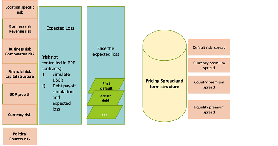
Diagram. The framework of component based model.
the construction is completed and moved into operation stage. Main project risk factors are included and reflected through business traffic revenue, operating cost and life cycle cost, financial capital structure, tax, and inflation etc., So all the risk factors can be accessed robustly through their impact on the project default, expected loss and credit risk pricing. In the case, the projected cash flow is considered as a base scenario.
In a typical project financing structure, while some risks such as construction or regulatory risks may be clearly controlled by the project participants, the traffic revenue risk may not be fully hedged by the PPP participants. The traffic revenue risk has often been one of the greatest challenges in project financing.
The transportation projects are particularly subject to a variety of financial risks due to the large initial costs, high irreversibility (sunk costs), extended contract duration, and high contract complexity due to the involvement of several parties with different objectives and constraints (Checherita & Gifford, 2007) . For transportation projects, appropriate mitigation of the financial risks by the project participants is one of the most critical success factors (Chiara & Garvin, 2007) . Many projects fail due to high levels of risks and the inefficient risk sharing mechanisms between the public and private sectors (Cuttaree, 2008) .
Then Monte Carlo simulation for cash flow CFADS is set up. In the implementation, industry parameter calibration is conducted for further DSCR simulation. The single base case scenario does not include the risk volatility of the underlying project cash flows and therefore cannot reflect the actual riskiness of the project and cash flow to debt. A stochastic Monte Carlo cash flow model is established to model the project cash flows and embedded risk characteristics.
The cash flow available to debt service (CFADS) can be obtained for each year using the formula below:
CFADS = Nominal Revenue − Operation & Maintenance Costs − Life Cycle Costs − Approx. Taxes
Debt service coverage ratio (DSCR) is defined as the ratio of CFADS to total debt service including principal repayment and interest rate payment in each period.
Basic stochastic variables assumptions: Distributions for the main driving variables like annual traffic growth in each period, operating costs per annum and life cycle costs per annum etc. are made to illustrate the mechanisms of the stochastic cash flow model. The main risk factor volatility parameters and DSCR are calibrated to industry external agency risk implied through empirical marginal defaulting probability. The implementation of this hypothetical case is calibrated to the empirical default probability in Moody’s project financing study December 2012 (please refer to “Infrastructure Default and Recovery Rates, 1983-20-12H1, Moody’s, 2012 ).
In the implementation, we include the stress testing of the driving factors of project default and their impact on the credit rating of infrastructure debt. As discussed in previous section, it may be very useful for project structuring and risk assessment. In many cases, to serve the purpose of enlarging the investor base through enhancing the project debt credit rating to a higher grade e.g., investment grade, project sponsors need to identify the driving factors which have impact on the default probability and take steps to mitigate some risk using risk mitigation instrument. As described above, the DSCR is used as technical default trigger in EDHEC model and the distribution of the DSCR can be used to determine the default probability profile. By running the sensitivity analysis against DSCR distribution, we can identify the factors which may explain risk variance of the DSCR and at what magnitude. E.g., the cost component is identified as a factor which has an important impact on DSCR distribution through sensitivity analysis. We can also quantify the impact of the volatility of the cost component on the DSCR. This can be done by looking at its impact on DSCR distribution and furthermore on the probability of default when increasing one standard deviation of the cost volatility. Based on the change of the default probability caused by the volatility of the cost component, together with an assumption on the recovery rate, the expected loss caused by the additional volatility of the cost component can be quantified. Sponsors may compare the expected loss and risk issuance premium for buying an issuance to mitigate some portion of the cost component risk so as to enhance the project rating (e.g., investment grade) and make decisions on whether to sell the risk and share it with some third party or retain the risk by issuing a bond with lower rating and paying a higher bond yield spread premium.
As specified in EDHEC framework, after cash flow Monte Carlo simulation, Risk measure-Debt Service Coverage Ratio (DSCR) simulation and defaulting is implemented based on the calibrated cash flows (please see EDHEC’s unlisted infrastructure debt valuation and performance measurement, 2014). Based on the calibrated asset volatility and financial structure volatility, DSCR calibration and simulation model may be implemented. According to the simulated DSCR distribution, the project defaulting events and other states under all the simulated paths can be obtained for each period.
Based on the simulated defaulting event according to DSCR distribution in each period for all the paths, the debt cash flow payoff functions is built. An assumption of recovery rate should be made according to the industry empirical observation data for project finance discounted debt.
Considering the situation that the purpose of this paper is mainly aimed to provide the valuation solution for institutional investors and that the restructuring option might not be the most efficient and cost effect option for institutional investors, the payment cash flows are assumed to be the discounted value of the recovered outstanding asset’s clash flows when a default occurs. For the specialized asset restructuring and management company, they may model and incorporate the restructuring option and analyze the debt value by replacing the recovery component with restructuring option and other exit events.
Finally, credit risk pricing model uses risk natural approach, calculates expected loss and derives credit spread term structure. In risk neutral asset pricing framework, the simulated cash flows are risk adjusted and the cash flows are discounted by risk free reference rate. In this study, swap LIBOR rate is used as a reference rate. By discounting all the outstanding debt payoff cash flows using risk free rate as of a specific period along each simulated path, expected loss and credit spread can be computed as of each future time. Here, the cash flows are the risk neutral cash flows generated based on the risk neutral volatility simulation. The expected loss is calculated as the difference between the average of the present value of the simulated cash flows along all the paths as of a specific date for all the future periods and the present value of the scheduled debt service cash flows as of the specific date. As stated in financial theory literatures (please refers to Merton (1974) and Black & Cox (1976) for risk assets valuation), credit assets are treated as two parts, risk assets and risk free assets. The difference between the values of the two reflects the risk embedded in the credit risk spread.
3.2. Implementation in a Transportation Project Case
For this study, a hypothetical case is built. In this case, a toll road is to be built. The project period is expected to be 25 years, with a construction period of 5 years. During the period from year 6 to year 23 (totally 18 years), the debt will be repaid. There is a tail period of 2 years from the year 24 to the year 25 when the debt is supposed to have been fully repaid. The tail period is considered as a kind of collateral in the sense that the cash flows may be used for debt restructuring when credit event occurs so as to mitigate credit risk at some extent. The total capital investment is $100 million, of which 70%, total amount of $70 million, is financed by debt and 30% by shareholder’s equity from project sponsor. The following describes the implementation of the model building blocks in each step discussed in Section 3.1.
3.2.1. Base Scenario with Projected Cash Flows
In this case, the project revenue is mainly driven by traffic volume and toll rate. Traffic volume is determined by base traffic plus an annual growth for each year. The base traffic without growth is projected around 3.2 million vehicles each year. The base annual traffic growth rate is projected to be around 2.6% to 2.8% for the first six year after the conduction is completed (year 6 to year 11) and declines to around 2% in the following 5 years (year 12 to year 16), thereafter it is reduced to around 1.7% to 1.2% during the last 9 years (year 17 to year 25). The toll rate includes real toll rate and inflation adjusted nominal toll rate. The real toll rate is derived from a traffic volume band matrix. Assume that there are three bands for the traffic volumes: 1 million to 1.5 million, 1.5 million to 1.75 million, and 1.75 million and above. Accordingly, the real toll rates are determined respectively at $2, $1.65 and $1.35. The nominal toll rate is obtained by adjusting the real rate with inflation. The year to year inflation growth is assumed to be 2.5%. Using the projected traffic volume and toll rate, we get the real revenue and inflation adjusted nominal revenue.
The cost mainly includes the following variables: Operation & Maintenance Cost (O & MC) and Life Cycle Costs (LCC). Assume Operating Costs per annum is $165 M, Life Cycle Cost per annum is $180 M, by applying the nominal toll rate to the cost, O & M and LCC can be calculated. The approximate tax cost is calculated with a tax rate assumption of 30%. The tax base is using nominal revenue subtracting O & MC/LCC and annual debt service amortization.
Finally, the debt service payments schedule is determined by amortizing the principle repayment during the period from year 6 to year 23 (18 years) and 6% of interest rate is assumed for the interest cost service payment occurred in each period.
According to the projection, The cash flow available to debt service (CFADS) under base scenario is around $3.5 million to $7 million during the period from year 6 to year 23 and the total debt service amount is around $3.2 million.
In a revenue availability based infrastructure project as this hypothetical project, the debt payment is mainly structured to have a slowly raising DSCR to meet the requirements from debtor for partially mitigation of the revenue risk. With the deleveraging of the project capital structure, the DSCR is around 1.2 and slowly grow to around 2.5 in the base case. The main cash flow variables and projected cash flows in base case for each 6 months period starting from period 1 (the first half of year 1) to period 50 (the second half of year 25) can be generated.
3.2.2. Monte Carlo Simulation: CFADS Cash Flow and Industry Parameter Calibration
In this case, for scholastics cash flows modeling, initial assumptions are made for the main variables. Specifically, assumption about the traffic annual growth rate in each period is a normal distribution with a volatility of 20% and a mean of the projected base value as given above in the base case; the assumption for Operating Costs per annum and Life Cycle Costs per annum is a normal distribution with a volatility of 8% and a mean of the projected base value.
Distribution of cash flows (CFADS): as shown in Figure 1, the simulated CFADS distribution in each period can be approximated as a normal distribution with an increasing mean and volatility. It can be mainly explained by the growing traffic and net
![]()
Figure 1. Distribution of cash flow CFADS.
revenue, and bigger accumulated volatility along a longer horizon. The mean ranges roughly from $3 million to $7 million and volatility is around 20%.
Distribution of Infrastructure Project Financing Risk Measure DSCR/Industry Parameter Calibration: As shown in Figures 2(a)-(c), under this hypothetical case and assumption with the main variables, the distribution of DSCR is approximately following a normal distribution in each period with a slowly growing mean and increased volatility. The mean of the approximated local normal distribution roughly ranges from 1.2 to 2.2 and volatility is about 10% to 20%. The first vertical line from left in Figure 2(c) represents the technical default trigger level and the area on the left represents the probability in the first period when DSCR is lower than the threshold (here assumed to be 1.1), that is, the project technically defaults. Other vertical lines in Figure 2(c) are made to illustrate the DSCR level where DSCR falls on the left to the trigger level with a certain probability (e.g., 5%) in very late periods. When sorting all the DSCR paths in Figure 2(c) for a specific period, the area which is on the left side to the DSCR technical default trigger vertical line (DSCR = 1.1) gives the probability of default in this period. Based on general industry practice, marginal probability of default can be calculated as the new default of the paths in each period conditional on that the same paths survived in the previous periods. Please see “ Moody’s (2006) paper: Credit Risk and Loan Evaluation” for the definition of marginal probability of default. The risk factor parameters can be calibrated to an industry empirical through mapping default probability based on DSCR distribution to external agency published empirical default probability.
3.2.3. Stress Testing of the Driving Factors of Project Default and the Impact on the Credit Rating of Infrastructure Debt
We discuss and illustrate the process and usage of the stress testing of the driving factors of project default through the example below and the impact on risk mitigating and credit rating enhancement.
Based on the DSCR distribution and the DSCR trigger threshold (assume 1.1) for technical default, we can calculate the default probability. In Figure 3(a), the derived default probability in this DSCR distribution is around 6% - 8% in the period after construction, which is higher than the external rating agency’s empirical probability of default statistics for investment graded project financing. In Moody’s (2010) industry study for project financing default and recovery, the default probability is around 2% - 3% in the first 5 year after the construction and then declines to a number which is very low, less than 1% (please refer to the paper: Moody’s (2010) , “Default and Recovery Rates for Project Finance Bank Loans, 1983-2008).
While both revenue risk and cost overrun risk factors are identified as main driving factors of DSCR distribution and the project default, normally, in an availability based project, the revenue risk would be categorized as commercial risk and retained in the project. Investors need to price in this risk when valuing the credit spread of the infrastructure debt or bonds. In contrast, sponsors may need to take measures to mitigate some of the cost overrun using risk insurance instrument to upgrade the project rating
![]() (a)
(a)![]() (b)
(b)![]() (c)
(c)
Figure 2. (a) DSCR distribution-mean, (b) DSCR distribution-standard deviation, (c) DSCR distribution.
to an investment grade to enlarge the investor’s base. This will have an impact on the distribution of DSCR and have the default probability reduced to be a level when mapping it to default probability empirical data. In Figure 3(b), the DCSR distribution is displayed for the project after some cost overrun risk volatility is reduced and mitigated using risk mitigating instrument or thirty party insurance. By uplifting and enhancing the credit rating of the project financing debt, the infrastructure debt or bonds may be financed through a larger investor base since the investment grade rating of the instrument may make the infrastructure debt to be included in legible asset classes for long term investors like Pension, Insurance and Sovereign Wealth Funds according to their investment guidelines.
The lower volatility of cost component would cause a CFADS/free cash flow with narrower dispersion and this characteristic is passed to and reflected in the DSCR distribution. As shown in Figure 3(b), after the partial mitigation of cost overrun risk, the DSCR would be shifted to the right a bit and dispersion is narrowed. According to the new DSCR distribution, the probability of default is reduced to around 3% - 5% after hedging some of the cost overrun risk. This cost risk volatility reduction can be achieved by using commercial insurance etc. The value of the insurance should be reflecting the expected loss component reduced by the default probability reduction. A certain recovery assumption is made for the expected loss calculation illustrates this impact. Figures (Figures 3(a)-(d)) show the DSCR distribution before and after cost component risk mitigation.
As an illustration, Figure 3(c) shows the DSCR distribution after the risk mitigation in one specific period. Figure 3(d) shows the distribution of free cash flows after risk mitigation, which has a narrower dispersion, and its mean is shitted to the right a bit. As shown in Figure 3(c), as an example, the DSCR has a lower probability of default reduced to around 5%. Through sensitivity analysis and testing, project sponsors may find an appropriate level and balance in terms of mitigating or retaining the risk through analyzing the relationship between the risk factor volatility and their impact on the infrastructure debt defaulting probability, and finally on the expected loss and credit rating.
3.2.4. Infrastructure Risk Measure―Debt Service Coverage Ratio (DSCR) Simulation and Marginal Defaulting Probability Term Structure
Based on the DSCR modeling and discussion in EDHEC paper 2014 and industry credit risk calibration with external rating agency’s empirical default probability statistics for investment grade project financing, assumptions are made for some major variables for DSCR simulation and project finance default model implementation.
In this hypothetical case for a toll road, the DSCR is calibrated to a lognormal distribution, with a mean reverting growth rate to 1.5% in the total project life cycle and 15% volatility of the growth. The starting value for DSCR is 1.3 and the volatility of the local normal distribution is 15% in the period 11 which is the period immediately after the construction is completed. As assumed above, a lognormal growth distribution for period 12 and thereafter is assumed.
Based on DSCR simulation, the marginal default probability which is conditional on the surviving of the previous period can be calculated for each period starting from year 6 to year 23 in this case. The details about the approximated local normal distribution of DSCR simulation are shown in Figure 4(a) and Figure 4(b).
Figure 5 and Figure 6 show the DSCR simulation results for some specific periods. Figure 5(a) shows the distribution of DSCR in period 11 (the first half of the year 6). The DSCR starts with this period as a local normal distribution. Technical default trigger: DSCR = 1.1; mean = 1.3, vol = 15% (annual); Default probability: 2.3%. As indicated, a lognormal growth distribution for period 12 and thereafter is assumed. Figure 5(b) shows the distribution profile of DSCR for period 12 (the second half of the year 6). It is shown that the DSCR’s distribution can be approximated as a local normal distribution. Technical default trigger: DSCR = 1.1; mean is 1.31, volatility is around 12%, Default probability: 1.4%.
To look at another point of the marginal defaulting term structure, the figures below plot the DSCR distribution and also give the approximate local normal distribution statistics for a later period, the year 7 (the second year after the construction) to make the analysis easier and more transparent. Figure 6(a) shows the distribution of DSCR in period 13 (the first half of year 7). Local normal distribution (approximatively) mean = 1.326, volatility = 15%. Default probability: 0.9%. Figure 6(b) shows the distribution of DSCR in period 14 (the second half year 7). Local normal distribution: mean = 1.326, volatility = 15% (annual). Default probability: 0.7%.
![]() (a)
(a)![]() (b)
(b)
Figure 4. (a) DSCR distribution-mean; (b) DSCR distribution-vol.
By calculating the marginal defaulting probability based on DSCR simulation for each period, we obtain the points for marginal defaulting term structure curve. DSCR calibration parameter indicated above is used for DSCR simulation. The marginal default probability curve is consistent with the empirical default probability statistics given in Moody’s documentation (please refer to the paper for more details, “Default and Recovery Rates for Project Finance Bank Loans, 1983-2011, Moody’s, 2012 ).
Marginal Default Probability and Cumulative Default Probability. Specifically, marginal default probability is calculated as below: taking the DSCR distribution of each period, computing the percentage of the DSCR events which are lower than 1.1 (technical default trigger). The new default is based on all the paths which have survived from the previous periods. According to DSCR simulation, sort all the surviving DSCR and count the new default among these surviving paths based on the DSCR technical default trigger. For illustration, the calculated marginal default probability term structure and cumulative default probability are shown in Figure 7(a) and Figure 7(b).
According to the calculated marginal default probability and cumulative default probability, three phases can be illustrated. Starting from the period just after the construction is completed, the year 6 and the default probability is more than 3% and
![]()
![]() (a)
(a)![]() (b)
(b)
Figure 5. (a): DSCR distribution in the first half of year 6; (b): DSCR distribution in second half of year 6.
slowly decline to around 1.5% until the year 10 within five years (five years after the construction is completed). Here, the default is triggered when the DSCR level is lower than the 1.1 technical default threshold. Then the new default probability (marginal default probability) further declines from 1.5% and reaches a lower level around 1% in the year 15 (10 years after the construction period); after that it is at a lower level and almost reaching zero, around 0.6% until 20 years and 0.2% after 20 years. The results are consistent with the external rating agency’s empirical default study data. In Moody’s industry study, for project financing default and recovery, the default probability is around 2% - 3% in the first 5-year after the construction and then decline to a number which is very low, less than 1%.
The pattern displayed is also consistent with theoretical study and industry empirical observations. When horizon is extending, the asset volatility is larger since the analysis
![]() (a)
(a)![]() (b)
(b)
Figure 6. (a) DSCR distribution in the first half of year 7; (b) DSCR distribution in the second half of year 7.
is projected to a longer horizon and the time scaling effect causes a bigger risk, when independent identity distribution (IID) is assumed for asset factors. The growing volatility of the asset are offset with an increasing speed by the deleverage of the capital structure. Marginal Default Probability (this is the chart title) Especially, in project financing, where the starting leverage is normally at a higher level, the impact of the deleveraging process would be high and more obviously observed compared with the
![]() (a)
(a)![]() (b)
(b)
Figure 7. (a) Marginal default probability; (b) Cumulative probability of default.
deleverage effect of typical corporate financing process whose starting leverage is normally moderate and not high. Please refer to the paper “Structural Credit Risk Modeling: Merton and Beyond”, Yu Wang, risk management, 2009 and the paper by Marco & Blaise (2004/2012) .
From another aspect, the mean and standard deviation profile of DSCR lognormal growth distribution and local distribution statistics may also help explain this trend of declining marginal default. Let us look at the approximated local distribution. The mean of DSCR starts from 1.3 and grows to about 1.6 in year 23 (within 18 years after the construction), with an average growth rate of 0.6% (staring from 0.2% to 1.5%). The volatility of estimated local normal distribution is growing from 12% in year 6 (the first year after construction) to 40% in year 23 (the 18th year after the construction). The skewness is also shown in Figure 5 and Figure 6. E.g., it is 0.388 for DSCR in period 12 (the second half of the year 6). It is then increased from 0.3 in year 6 to around 1 in year 20. The general declining of DSCR is reflecting the effect of the deleverage and the deleveraging may offset more the impact from higher volatility in longer horizon.
3.2.5. Debt Cash Flow Pay-Off Function and Cash Flow Simulation
Based on the simulated DSCR and CFADS along different path, the cash flow available to debt can be determined. As an illustration, for example, as Figure 8(a) shows, in the first half of year 8 (period 15), under 5.3% of the paths, which is the area on the left side, the simulated debt service (cash flow payment) is 0. These paths reflect the defaults in the previous periods. In one period, if the project defaults under a path, the
![]() (a)
(a)![]() (b)
(b)
Figure 8. (a) Debt payoff distribution in the first half of year 8; (b) Debt payoff distribution in the second half of year 21.
debt payoff function gets an amount which is the recovered rate multiplied by the total outstanding cash flows in that period. E.g., in the period of 15, the total amount of the outstanding cash flows as of the first half of the year 8 is $97,638,222, 355 and no cash flows occur in the following periods (the period 16 and all the later periods in the project cycle) along these paths which default. In Figure 8(a), the 0.8% of path which is the area on the right reflects the new default in the current period, the period 15 (the first half of year 8). Under these new default paths, the debt flows as of the first half of the year 8 is $97,638,333. Under the rest of the paths (around 96%, the middle part in the figure), the debt service cash flows are the regular scheduled principal and interest payment for the current period, the period 15, which is $3,126,667. For a later period, the accumulative effect of the defaults which occurred in the previous periods can be observed more obviously. Figure 8(b) shows the debt payoff cash flows distribution for period 42 (the second half of the year 21). In this period, the scheduled debt payment is $3,153,888, the total amount of the outstanding cash flows of the futures period as of the date in period 42 is $12,518,333. In this figure, 15.9% of the paths represent the accumulative defaults which occurred immediately after the construction until the period 42. Under these 15.9% of the default paths the cash flows for debt service are zero as of period 42 (year 21). As stated before, in each period, if there is a default, the cash flows for the future periods under these paths are stopped and set to zero, the recovered cash flows (assumed to be 40% of the total outstand cash flows) are put in the current period when the new default occurs in the current period.
3.2.6. Credit Risk Pricing Using Risk Neutral Approach/Calculating Expected Loss and Deriving Credit Spread Term Structure
Credit risk asset valuation and hump-shaped credit spread term structure for project financing bonds/debts.
As described in EDHEC framework, after we have DSCR simulation and simulated default events, we can simulate debt service cash flows for all the paths. If there is a default, generate the cash flow as the recovered rate multiplied by the outstanding cash flows; then discount the cash flows in each period for each path using the simulated interest rate model rate for a risk free reference proxy (LIBOR swap rate is used for this study to illustrate the mechanism) and get the present value of the simulated debt service cash flows. In this asset pricing model implementation, Hull-White modeling is used for interest rate simulation. The expected loss is calculated as the difference between the average present value of the total present value of the simulated debt pay off cash flows with the total present value of the debt service cash flows.
Based on the simulated debt cash flows as described in above, we can evaluate debt, calculate the expected loss and credit spread. E.g., for the spread as of year 10, the discounted PV as of the year 10 of the recovered cash flows for the default paths and the discounted value of the cash flows for the live paths will be summed up. The expected loss as of year 10 can be calculated as the difference between the PV of the simulated cash flows and the PV of the debt scheduled service. The other points on the credit spread term structure curve are estimated using the similar way. The hump-shaped credit term structured curve generated is displayed in Figure 9 for illustration purpose. According to the paper by Ehler from BIS, the empirical credit spread is about 200 bps during the 5 year and the expected loss derived spread from the model is around 200 - 250 bps around year 5 when the construction is done. Credit term structure curve results will be further discussed in section IV. Figure 10 shows the empirical credit spread of project financing debt in the study conducted by research paper from BIS. Please see more details from the paper by Marco & Blaise (2004/2012) , “The term structure of credit spreads in project finance”, and “Understanding the challenging of infrastructure financing” (BIS, 2014) . Figure 11 gives some analysis conducted by
![]()
Figure 9. Modeled credit spread term structure evolution. Source: own model.
![]()
Figure 11. Project financing bonds information (Barlcays Capital Summary). Source: Barclays/European securitization mid-year outlook, 17 June 2013 45, PROJECT FINANCE.
Barclay’s capital about the market credit spread for project financing based debt for information purpose. These projects have a spread between 130 bps to 250 bps depending on the different rating and project structures.
We use an example to further illustrate the deriving of a credit spread point. On the credit term structure curve, the forward credit spread is calculated by discounting the simulated debt cash flows using the simulated interest rate as of future date using Hull White interest rate model. E.g., for the credit spread on year 6 (the first year after the construction), the risk neutral cash flow has about 6% of 1000 paths under which the project default (risk neutral default probability), the expected loss is about 200 bps as a percentage of the scheduled debt service value as of year 6 give some analysis on the analysis conducted by Barclay’s capital about the market credit spread for project financing based debt for information purpose.
4. Modeling Result Discussion
DSCR simulation: As discussed before, to establish a robust industry asset and defaulting model for project finance debt, the asset volatility and financial structure volatility should be calibrated taking the industry empirical data level into consideration so that the marginal defaulting probability can be mapped with the external agency’s empirical default probability for a specific industry sector and credit rating. In this hypothetical case for a toll road, the project marginal default probability of project is calibrated to Moody’s empirical default probability for a universe of project financing loans.
Here, the DSCR is assumed to follow the similar distribution with the project financing underlying assets. In Merton’s model, lognormal assumption is assumed for company asset with a constant volatility of growth. Under some recent modeling approach, time varying volatility for the asset life cycle or stochastic volatility model have been analyzed (e.g., please refer to Heston Model for stochastic equity modeling). In our calibration model, the project financing asset is modeled through a lognormal distribution with a mean reverting growth to reflect more information about the nature and risk characteristic of project financing.
Based on DSCR simulation, the marginal default probability which is conditional on the surviving of the previous path can be calculated for each period starting from the year after construction until the end of project cycle, which is the year 6 to year 23 in this case. The parameters and assumptions are calibrated as below according to the empirical defaulting probability study “Default and Recovery Rates for Project Finance Bank Loans, 1983-2011, Moody’s, 2012. Specifically, DSCR is calibrated to a lognormal distribution, with a mean reverting growth rate to 1.5% in the total project life cycle and 15% volatility of the growth. Its current level of growth is 0.2%. The starting value for DSCR is 1.3 and the volatility of the local normal distribution is 15% in the period immediately after the construction is completed. The DSCR trigger for technical default is assumed to be 1.1 as an illustration of the mechanism. Other defaulting logics can be applied. This calibration is just to illustrate the mechanism designed in this model framework and does not serve to provide an indicative spread. The DSCR has a profile with a slowly growing mean and increased volatility to reflect the situation that a commercial availability-based project is structured to deleverage gradually to meet the risk controlling demand from debt investors as project participants.
Marginal Default Probability and Cumulative Default Probability. Three phrases are displayed in the marginal deflating probability term structure, as shown in Figure 7(a) and Figure 7(b). Starting from the period just after the construction is completed, year6 in this case, the default probability is more than 3% and slowly decline to around 1.5% until the year 10 within five years (five years after the construction is completed). Here, the default is triggered as the DSCR level is lower than the 1.1 technical default threshold. Then the new default probability (marginal default probability) further declines from 1.5% and reaches a lower level around 1% in the year 15 (10 years after the construction is done), after that it is at a lower level and almost reaching zero, around 0.6% until 20 years and 0.2% after 20 years. The results are consistent with the external rating agency’s empirical default study data. Please see the industry study by Moody’s, 2012 for project financing default and recovery. As discussed previously, the mean and standard deviation profile of DSCR lognormal growth distribution and local distribution statistics may explain this trend of declining marginal default. The general declining of DSCR is reflecting the effect of the deleverage. And the deleveraging may offset more the impact caused from more wide disbursed distribution when volatility has increased within the longer time horizon.
Credit risk asset valuation and hump-shaped credit spread term Structure for project financing bonds. The credit term structure curve is derived based on DSCR simulation defaulting model and expected loss calculation. As shown in Figure 9, the credit spread term structure is consistent with the empirical project financing debt term structure shown in Figure 10. Please refer to the research paper of Marco & Blaise (2004/2012) “The term structure of credit spreads in project finance”, and BIS (2014) . The spread is around 200 bps for investment grade debt in the period after the construction according to these empirical studies. As shown in Figure 10, in the hypothetical case we are studying, the credit spared calculated by the model is around 200 - 250 bps. The hump- shaped profile is observed in the empirical study. It reflects the deleverage process of the financial structure in project financing project. The Merton model can be used to illustrate this effect through the analysis of the evolution of the credit spread term structure. Please see paper by Wang (2009) “Structural Credit Risk Modeling: Merton and Beyond”, Risk Management, Several industry empirical study papers also have analyzed the driving forces for the humped credit term structure, which can be an obvious feature for project financing where the deleverage is highly conducted through the period after construction. Please also see the paper by Marco & Blaise (2004/2012) about Credit Term Structure of Project Financing and EDHEC 2014 paper about Unlisted Infrastructure Debt Valuation and performance measurement. This credit curve reflects the credit risk in terms of making debt service payment by sponsor including both principal and interest payment. For infrastructure project financing (limited recourse), the creditness is purely backed by the project assets cash flows themselves. The project financing risk factors may include business risk from revenue risk and cost overrun risk, political risk, FX risk etc. Project financing can be treated as a package of contracts within which the risk factors are specified. Some of the risk factors are retained by the sponsor like business revenue risk, some of the risk may need to be mitigated and shared with external insurance through credit risk enhancement instrument. The risk sharing and allocation are structured in a way based on the risk bearing capacity of each parties including sponsor (most likely shareholder), infrastructure bond/ debt long term investors, insurers to maximize the money value of the project and social wealthy. When there is a market failure where there is inconsistency between the incentive and the role and function of different types of capital participating in the long term investment, credit enhancement instrument or other de-risking mechanism with public financial support need to be utilized to provide the market based risk and return characterizes of the infrastructure long term debt, so that the project would be commercially valid.
5. Conclusion
The component-based valuation model framework and implementation building blocks provide a robust platform and tool, which will allow investors or issuers to make informed decision to make a choice of risks to retain, pass through or take mitigation actions according to their preference and risk taking capacity. This is a crucial step towards the establishment of infrastructure asset as a separate, transparent and harmonized asset class which may be attractive to long term investors. The project financing credit spread curve derived from this platform is aimed to help investors or issuers to access the pricing component of the infrastructure project debt using ex-ante risk basis. By using the DSCR risk measure and credit risk pricing building blocks, the model tool can be extended and applied to risk management and portfolio construction, infrastructure debt structuring and product innovation. E.g., when using infrastructure market based or government-based product innovation to mitigate refinancing and construction risk, the investor or issuer may assess the value of alternative options which allow the investors to invest in the infrastructure debt at different time period of the project cycle, at time zero vs. a future date. In order to greatly enhance the accessing capacity of the long term intuitional investors to infrastructure investment, an industrialized investment benchmark process for main infrastructure sectors may be set up using the tool and external agency empirical default data for project financing.
Acknowledgements
We are very thankful to the participants’ useful discussion from the World Bank MOCC Finance for Development, and the brain storming discussion on Infrastructure Investment in Emerging Markets organized by Fiona Elizabeth Stewart. We are very thankful to Mr. Majid Hasan for the helpful discussion.
Disclaimer
The paper represents the authors’ view. The findings, interpretations, and conclusions expressed in this paper do not necessarily reflect the views of the Executive Directors of The World Bank or the governments they represent. The World Bank does not guarantee the accuracy of the data included in this work. The boundaries, colors, denominations, and other information shown on any map in this work do not imply any judgment on the part of The World Bank concerning the legal status of any territory or the endorsement or acceptance of such boundaries.
NOTES
1http://www.ppiaf.org/sites/ppiaf.org/files/publication/PPIAF-Institutional-Investors-final-web.pdf