A Comparative Study of Two Spatial Discretization Schemes for Advection Equation ()
Received 29 December 2015; accepted 5 March 2016; published 8 March 2016

1. Introduction
A currently active area of research is the numerical solution of nonlinear partial differential equations and nonlinear integral equations [1] -[7] . An advection equation is fairly in shape but it is one of the most difficult equations to approximate numerically.
The nonlinear advection equation arises in various branches of physics, engineering and applied sciences. The importance of obtaining the exact or approximate solution of this equation is still a significant problem that needs new methods to discover exact or approximate solution.
The linear advection equation is simple in form and yet it is one of the most difficult equations to solve accurately by numerical means [8] . This equation is challenging to solve as it causes some discontinuities with neither dispersion nor dissipation. However, all efforts to use a fixed number of space intervals will result in both dispersion and spurious oscillation. The use of traditional symmetric techniques is possible only if the terms of arbitrary second order artificial viscosity or damping are introduced to the equation. Directional (or upwind) methods have shown to be efficient for the purpose of finite difference analyses as it clears the oscillation problem, yet they will not remove it completely. The linear advection equation does provide a good case for testing methods to be used on systems of hyperbolic equations. Many schemes have been tested on it, generally by using propagating step, sine, Gaussian or triangular waveform [9] . These techniques were used to provide a rational for choosing a spatial scheme for first-order hyperbolic equations. The optimal choice is not invariant, but depends on the application.
In this paper, the advection equation is solved by finite difference method [10] [11] and the stability conditions for the scheme are also discussed. Numerical finite difference scheme is developed for obtaining approximate solution to an advection equation using the 3-point formula introduced in [12] . The same problem is considered using modified method of lines [13] -[15] , with a new three-point difference [12] . Using this new difference leads to stable schemes for the two methods. Numerical results are shown and compared with analytical solutions.
2. Finite Difference Method with a Good Spatial Discretization
Let us consider the equation
 (1)
(1)
and v is a nonzero constant velocity, where  with the initial condition
  The finite difference method begins with discretization the space variable x and the time variable t as follows
 ; and
; and .
.
The using of some of the finite difference schemes on advection equations can cause unstable solutions. To add stability, upstream (backward or forward) could be used for spatial discretization for the first-order differences. However, for a given spatial accuracy, these differences need to use extra grid points than centered difference. An artificial dissipation (or viscosity) term is normally introduced to a central differencing scheme for stability reasons but it is not easy to determine the magnitude of this term required for the stability and effect of this term on the solutions.
The aim of new method is to develop a good formula with high accuracy for the numerical solution of the advection equation using the spatial discretization presented by Sharaf and Bakodah, [12] , using 3-points formula, thus the approximate form of the first derivative is
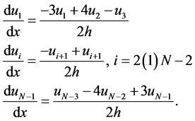 (2)
(2)
Adopting a forward temporal difference scheme, this yields
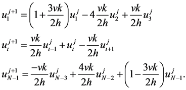 (3)
(3)
There are two standard methods of the finite-difference equation. In the first method, a finite Fourier series is used. In the other method, the equation is expressed in matrix form, and the eigenvalues of the associated matrix are examined. In order to investigate the stability of this scheme by the first method (Von Neumann stability analysis), it is considered
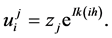 (4)
(4)
Replacing  in relation (2) from (3), it is obtained:
 (5)
(5)
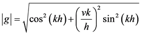
where
 (6)
(6)
The stability condition  is fulfilled for all k as long as,
 (7)
(7)
 (8)
(8)
That is, the method (2) is stable.
3. Modified of the Method of Lines
In the Numerical Method of Lines (NMOL), the partial differential equation (PDE), to be solved, is transformed into a system of ordinary differential equations (ODEs) by discretizing all the independent variables but one [16] . The advection equation, depending on time t and one spatial variable x, either t or x can be discretized, and the integration will be carried out along the remaining undiscretized independent variable.
The technique consists of converting the PDE into ODEs either by finite difference spline or by weighted-res- idual technique, then integrating the resulting ODEs [17] . Finite differencing in the spatial variable led to a set of timedependent ODEs. The advantage of using (NMOL) is that sophisticated software packages exist for the numerical solution of ordinary differential equations. These software packages contain iterative methods for handling non-linearities and feature automatic step-size adjustment and integration order selection to maintain a specified error and to solve the problem with near optimal efficiency. Several recently software packages for automated method of lines solution of arbitrarily defined PDEs have been very successful, particularly for parabolic and elliptic PDE systems.
Such facilities can be improved for hyperbolic equations by incorporating an upwind weighted residual technique. This technique is similar and superior to the use of an artificial viscosity term, and it could be implement easily in any software package. Previous considerations of the (NMOL) to solve PDEs have been geared to parabolic equation and generally used centered, second-order differences. Using these differences on hyperbolic equations can lead to unstable solution. To add stability, upstream (backward or forward) first-order differences could be used for the spatial discretization. But these differences require the use of more grid points than central differences for a given spatial accord. An artificial dissipation (or viscosity) term is often added to a central differencing scheme to add stability but it is difficult to determine the magnitude of this term required for the stability and the effect of this term on the solutions. Other stabilizing techniques that have been employed in the explicit finite difference procedures are generally not applicable to the method of lines approach because they involve manipulation of terms in both the time and space discretization.
In this paper, a modified method of lines using a new three-point difference [12] is used. The use of this new differences leads to stable schemes with good accuracy. In order to apply the method of lines to the advection equation (1), the spatial derivative must be approximated. An equally spaced mesh  is used. As in the Ref. [12] a new difference scheme can be used in the calculation of
 ![]()
![]() (9)
(9)
It leads to stable schemes with good accuracy. In this section the second method shall be used. The analysis of eigenvalues of the system gives the necessary conditions for the stability of discretization of the problem [18] . The stability corresponds to real and negative values.
By considering equation (1) with the centered difference scheme of order two, then we get
![]() (10)
(10)
where ![]() is
is
![]() (11)
(11)
and![]() .
.
Mathematically the difference scheme is stable if there exists a real positive eigenvalues. However, where ![]() is a tri-diagonal matrix, the corresponding eigenvalue
is a tri-diagonal matrix, the corresponding eigenvalue ![]() of A can be calculated from the relation.
of A can be calculated from the relation.
![]() (12)
(12)
where![]() . Thus
. Thus
![]() (13)
(13)
which are pure imaginary values.
So, we consider the non-centered formula approximation
![]() (14)
(14)
with the matrix formula ![]() where
where
![]() (15)
(15)
Thus the eigenvalues are given by
![]() (16)
(16)
These values are real and negative, so the difference scheme is stable.
4. Numerical Examples
4.1. Example 1
We apply the Finite Difference Method with a good spatial discretization to solve linear advection equation to demonstrate the validity of this method.
Consider the equation
![]() (17)
(17)
with the conditions
![]()
With the analytic solution
![]()
Using equation (3) we find
![]()
let
![]()
Table 1 shows the absolute error ![]() for the finite difference method in different value of time.
for the finite difference method in different value of time.
4.2. Example 2
We apply the Modified of the Method of lines to solve linear advection equation to demonstrate the validity of this method.
Consider the following advection equation
![]()
with the conditions
![]()
Table 1. Absolute errors of the finite difference method, where![]() .
.
![]()
and the analytic solution
![]()
Substituting in equation (9) we find
![]()
and the condition are
![]()
Hence, we can write
![]()
So, to confirm the accuracy and efficiency of the method, the absolute error ![]() are used (Table 2).
are used (Table 2).
4.3. Example 3
Consider the equation
![]()
and
![]()
with the analytic solution
![]()
Table 2. Absolute errors of the modified of the method of lines where![]() .
.
![]()
In this example we apply the Modified of the Method of lines and the finite difference method to solve linear advection equation to demonstrate the validity of them and compare between them.
Table 3 shows the absolute error ![]() for the finite difference method equation (2), and the method of lines.
for the finite difference method equation (2), and the method of lines.
4.4. Example 4
Consider the advection equation
![]()
with the condition
![]()
and the exact solution
![]()
This problem is solved for![]() , with
, with![]() .
.
Table 4 shows the absolute error ![]()
![]()
Table 3. Comparison of the absolute error between finite difference method and the method of lines, for example 1 with![]() .
.
![]()
Table 4. Comparison of the absolute error between finite difference method and the method of lines, for example 2 with![]() .
.
5. Conclusions
From the studied test examples, it has been found that, the modified method of lines gives better results than the finite difference method. Although the modified method of lines is used to approximate the first order hyperbolic differential equation. Thus equations are one of the most difficult classes of PDEs to integrate numerically. To overcome this, a modified MOL scheme is suggested. The results are in good agreement with the exact solution as shown in Table 1, Table 2. The presented method is attractive for hyperbolic, parabolic and elliptic equations.
The methods introduced in this paper for solving the linear and nonlinear advection equation are based on finite difference method. The best choice of the numerical method for a given problem depends on the stability condition.