A Practical and Automated Hall Magnetometer for Characterization of Magnetic Materials ()
1. Introduction
During the last decade, scientific research on the diverse magnetic properties of bulk materials, particles, microparticles, and nanoparticles has been adequately supported by various new and sophisticated characterization techniques. Properties like the Curie temperature, saturation magnetization, coercivity, magnetic anisotropy, and polarization rotation are some of the most important parameters for magnetic materials that guarantee their applications [1] -[3] . Various techniques, such as superconducting quantum interference device (SQUID), vibrating sample magnetometer (VSM), Mössbauer spectroscopy, magneto-optic Kerr effect (MOKE), torque magnetometers, ferromagnetic resonance and Hall magnetometer, have been used successfully to study magnetic materials in the bulk form and magnetic nanoparticles [4] -[10] .
Among the sensing technologies used, the one based on the Hall effect has played an important role owing to its ability to measure dc fields (i.e., constant in time), large frequency bandwidth, non-hysteretic behavior, operation at high magnetic fields, reliability, and low cost. Traditionally, Hall magnetometry has been performed without the use of moving parts [11] -[14] .
In this paper, we present a different approach to measuring magnetization curves: a Hall magnetometer built from various equipment that is usually available in most laboratories, such as a Hall effect sensor, a small electromagnet, a current source, a voltmeter, and a linear actuator. One advantage of this magnetometer is its easy assembly and customization. The nucleus of the magnetometer consists of a small acrylic camera, which works as an electric device for the electromagnet poles, and it is built with a path to guide the sample. We used a low- cost GaAs Hall effect sensor as a magnetic sensor. A model that considered the geometry of the sample was developed in order to increase the precision of the obtained magnetic moment. The magnetometer resolution was limited by the employed Hall sensor to 10−8 Am2 and recorded the magnetic hysteresis loop up to 1 T at room temperature. The device was calibrated independently and its performance was compared to that of commercial VSM (LakeShore, model 7400) and SQUID (Quantum Design, MPMS-XL) magnetometers, showing errors smaller than 1.7% in the magnetization obtained for various samples. All the equipments involved in the operation of magnetometers were controlled using LabVIEW®.
2. The Hall Magnetometer
2.1. Structure
In VSM magnetometers, the sample vibrates at a specific position, in contrast with this type of magnetometer. The Hall magnetometer must move the sample during the measurement; for this purpose, it requires a track from the sample to move in constant form, and the reading is simultaneously acquired by the Hall effect sensor. The configuration of the magnetometer is illustrated schematically in Figures 1(a)-(d).
Thus, the first restriction is to ensure the homogeneity of the magnetic field applied by the electromagnet (GMW 3470). In order to achieve at least 0.1% homogeneity, the employed electromagnet (with poles of 40 mm in diameter) has a distance of 5.3 mm between the poles to allow the displacement of the sample, which is approximately mm from the center of the poles along its diameter (see Figure 1(a)).
A Hall effect sensor (model HG-166A) with dimensions 2.5 mm × 1.5 mm × 0.7 mm is located on the holder with its plane perpendicular to the shaft fastening. According to the direction z shown in Figure 1(b), to measure the magnetic field applied by the electromagnet we used a Gauss meter (F. W. Bell, model 5080) to obtain the calibration curve in units of T/A; this approach relates the magnetic field in the region between the poles of the electromagnet to the current applied by the source. The electromagnet is supplied by a programmed power supply configured in current mode (Agilent 6654A), which can supply positive current outputs up to 9 A with steps of 3 mA in its smaller scale. A threshold current of 5 A was used to ensure a safe margin for the operation of the electromagnet. At the sides of the sample holder, two holes of 45 mm in diameter accommodate the electromagnet poles. At the front, a groove of 5.3 mm functions as a track to guide the sample holder. At one of the ends of this sample holder, there is a cylindrical cavity with its axis aligned with the x axis of another cavity, which is located at the other end of the z axis (Figure 1(c)). The cylindrical cavity is filled with magnetic material and is placed a few millimeters away from one of its ends in the positive direction of the axis (Figure 1(d)), in order to maximize the flux induced by the Hall effect sensor.
The Hall sensor has a magnetic field resolution of 600 nT and an active area of approximately 1.26 10−7 m2 [15] , which is located 0.25 mm away from the bottom of the package sensor. The sample holder is pushed and pulled by a linear actuator in 0.5 mm steps. Small steps are possible; however, this would increase the total measurement time. A single digitization operation is performed for each value of the magnetic field in about 10 s by the reading system.
![]()
Figure 1. (a) Shematic of the Hall magnetometer. (b) Top view of the track and sample holder. (c) Lateral view of the track and sample holder. (d) perspective view of the Hall magnetometer.
2.2. Reading System of the Magnetic Field
To optimize the Hall sensor for readings of the magnetic field induced in the sample, we must determine the feeding current sensor. We conducted a study of the behavior of the signal noise of the sensor for various values of applied current (Figure 2(a)) using a spectrum analyzer. We applied a known magnetic signal (70 µT at 4 Hz) and supplied the Hall sensor with four different currents: 1.0 mA, 2.5 mA, 5.0 mA, and 7.0 mA. The measured spectrum verified that below 1 Hz, the lowest-intensity noise corresponded to a current of 5.0 mA. In this case, the reading of the spectrum analyzer was approximately 0.63 µT.
Tests were performed in the presence of magnetic fields. The results of one of these tests (Hall sensor measurement in the presence of a magnetic field of 335 mT), displayed in Figure 2(b), demonstrated that the sensor was sensitive to the applied magnetic field, even with its axis of sensitivity perpendicularly aligned with the electromagnet axis. However, the applied magnetic field did not significantly degrade the performance of the sensor. Its sensitivity was only reduced in approximately 5% for an applied field of 335 mT. In Figure 2(c), we demonstrate that the Hall sensor has negligible hysteresis.
A current of 5 mA was then applied to the Hall sensor using a programmable current source (Keithley, model 6220) for the reading of the detected magnetic field. This source has a precision of 0.05% and a resolution of 100 nA in the range from 2 mA to 10 mA [16] . The response of the sensor to this current was measured by a voltmeter with two channels for different band readings. Channel 1, which was used to measure in the 100-mV full scale, has a resolution of 10 nV And can read continuous and alternating voltages in the band from 3 Hz to 500 Hz [17] .
Therefore, the reading system consisted of a current source and a voltmeter that were integrated in a system called Delta Mode and communicated with each other using an RS-232 connection and a trigger signal.
The current source applied a square wave of pre-defined amplitude (±5 mA) to the sensor with a frequency of 100 Hz and provided a nanovoltmeter with the timing information of the signal through the trigger. After reading the signals from several consecutive cycles, the nanovoltmeter calculated the mean and communicated the
![]()
Figure 2. (a) Measurement results demonstrating the relation between the signal noise of the Hall sensor and the applied current; (b) Hall sensor response in the presence of a 335-mT magnetic field; (c) Magnification of Figure 2(b) near the zero field.
result to the current source through the RS-232 connection, which sent this information to the computer via GPIB.
3. Calibration Procedure
Although the VSM magnetometer can also be used for absolute measurements, in practice, it is typically implemented for calibrations through the comparison with the magnetization patterns measured for a nickel sphere in a high field. The SQUID magnetometer usually needs to be calibrated by the final user [18] .
In the constructed Hall magnetometer, we used 99% pure nickel spheres with a 3 mm diameter in order to perform the calibration independently from the other magnetometers. The magnetization results were compared to values obtained using the same spheres in the two commercial magnetometers. In this case, we used a magnetic dipole model placed at the center of the sphere, which coincided with the center of the sample holder. Before obtaining the value of magnetization, we used the spatial dependency of the magnetic dipole model to determine the distance between the center of the sample holder and the center of the Hall sensor. According to Figure 1(a), the induced magnetic moment is oriented along the x direction and the component of the magnetic field is measured along the z direction.
The proposed model for the calibration of the nickel sphere was a magnetic dipole located at the origin of the system of coordinates, with a magnetic moment mx pointing to the positive direction of the x axis. The center of the sensor was at the position (x, y, z) = xi, yj, zk.
The equation that represents the magnetic field produced by the point magnetic dipole is:
 (1)
(1)
Because the magnetic moment was oriented in the direction of the x axis: m = mx i. Simplifying Equation (1), the equation used for the construction of this model is:
 (2)
(2)
The magnetic flux from the z component of the magnetic field of a dipole through an area π² is given by [19] :
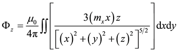 (3)
(3)
where x, y, z represent the coordinates of the sensor in relation to the dipole. The dipole is located exactly in the region between the poles of the electromagnet, thus defining the sphere to be analyzed.
This sphere is displaced in the y direction (negative), the greatest intensity of the magnetic field occurs when the sample passes by the sensor, out of its center. According to Equation (2), the unknown values are x, y, z, and mx. The value of ymax can be determined through the region of maximum intensity of the magnetic field read by the sensor.
We can substitute the integral calculation in Equation (3) using the reciprocity principle, which estimates the  flux produced by the magnetic moment of the dipole that passes through the area of the Hall sensor by:
 (4)
(4)
where  is equal to the field produced at the position of the dipole by a fictitious coil with its center located at (x, y, z), the center of sensor, and with a radius equal to that of the coil when excited by a unit current; m is the dipole magnetic moment. We only needed to calculate Br, which can be written in terms of complete elliptic integrals of the first and second kind (K and E, respectively) [20] .
where  and as represents the radius of the fictitious coil,
 and
and
Because only mx differs from zero, we can calculate Bx as:
 (5)
(5)
The magnetic flux of the x-component of the magnetic field of a dipole through an area is given by:
 (6)
(6)
The calibration process of the Hall magnetometer begins by obtaining the distance from the center of the sample holder to the center of the Hall sensor. These values are subsequently used to determine the desired magnetic moment. The values of x0 and z0 used in the dipole model (Equation (6)) represent the horizontal and vertical distance, respectively, from the center of the sensor to the center of the sample.
To determine x0 and z0, we used a sample holder with two cylindrical cavities, where we two nickel spheres of equal mass (126 × 10−6 kg) were placed. These were positioned at a distance of 22.5 mm in relation to the other (minimum distance required to avoid influencing each other’s induced magnetic fields, see Figure 3). They were placed in different positions, x0 and z0, in relation to the center of the sensor.
Since the examined magnetization value is independent from the spatial dependence of the field induced in the spheres, we can normalize the measured magnetic field and only consider the relative distances between the spheres and the sensor. If we measure precisely the values of dz1, dz2, and dx2, we have a system of two equa-
![]()
Figure 3. Sample holder used in the calibration.
tions, corresponding to the two measures, and two variables, the distances x0 and z0.
Analyzing this sample holder in an optical microscope we can determine the values of dz1 and dx2 (Figures 4(a)-(d)). Once the relative distances are obtained, we denormalize the measures and obtain the desired magnetic moment. In this study, we repeated this procedure many times and obtained the average values x0 = 1.63 mm and z0 = 3.02 mm. It must be noted that these values were obtained considering the flux through the area of the sensor.
In the literature, the saturation magnetization of nickel occurs approximately at 0.5 T and has the value 55.18 Am2/kg at room temperature [21] [22] . This saturation value is for pure nickel; however, the nickel used in our calibration process was 99% pure.
Figure 5 shows a comparison of the magnetization measurement results obtained with the Hall magnetometer (circles), the SQUID magnetometer (red solid lines), and the VSM device (black solid lines) for the same nickel sphere as a function of the applied field.
For the maximum field, 1 T, the Hall magnetometer obtained a magnetization of 55.38 Am2/kg. For the same field, the VSM device measured 54.94 Am2/kg and the SQUID magnetometer 54.42 Am2/kg.
The difference in the magnetization curves was 0.8% and 1.7% in relation to the values obtained by the VSM and the SQUID magnetometers, respectively.
It is worth noting that our result was obtained independently from the measurements with the other magnetometers. Regarding the precision of our magnetometer, after repeated many times measurements performed during several months, we noticed that the standard deviation was 1.2%.
The automation of the Hall magnetometer was achieved using a LABVIEW program (Figure 6), which acquired and analyzed the data transferred from the reading systems to a computer via the GPIB interface.
4. Experimental Results
4.1. Nickel Microparticles
After the sample holder calibration, we removed the nickel sphere and placed the magnetic material in the cylindrical cavity located at the end of the sample holder.
We can observe in Figure 1(c) that this cavity is near the sensor, which prevents the use of the dipole model. For the calculation of the magnetic moment of the sample, it is therefore necessary to apply a different theoretical model, which should be adapted to the geometric characteristics of the system. Since the cavity of the sample holder is cylindrical, we used a current cylinder as a model of the sample. To express the component z of the corresponding magnetic field, we first analyzed the simplest case, which is a current ring located at the center of the cartesian coordinate system. We have:
 (7)
(7)
According to Equation (7), the Bz component for a cylinder of length L is:
 (8)
(8)
After establishing the geometric parameters, we need to determine the magnetic moment m of Equation (8), which adjusts the model to the experimental measurements. Using the data acquisition program developed with LabVIEW® (Figure 6), we can measure the response of the induced field of the nickel microparticles (this was obtained from a NiO reduction process). To each magnetic field values, the sample percure a fixed distance and
![]()
Figure 4. (a) Optical microscope measurement of the distance dz2; (b) Measurement of the distance dx2; (c) Measurement of the distance dz1; (d) Figure indicating the position of the sensor and the first cylindrical cavity with a nickel sphere.
![]()
Figure 5. Comparison of the magnetization data for a nickel sphere obtained with the Hall magnetometer (circles), the VSM device (black solid lines), and the SQUID magnetometer (red solid lines).
generates an induced field curve versus distance traveled, where each curve was optimized by the cylindrical model. By adjusting each of these curves, we can obtain the magnetic moment of the sample for each applied magnetic field.
As an example of the application of the cylindrical model, Figure 7 shows the lowest measured magnetic moment for the nickel sample, which was 2.12 × 10⁻⁵ Am2. Figure 7 compares the magnetization results obtained with the Hall magnetometer (blue circles) for 11.9 mg of nickel and those measured with the SQUID magnetometer using 2.2 mg of the same sample (red solid lines). By comparing the two magnetization curves, we obtained a mean square error of 0.43%; this is in accordance with the predicted magnetic moment measurement error for this sample holder.
![]()
Figure 6.LABVIEW program used for the automation of the Hall magnetometer.
![]()
Figure 7. Comparison of the data acquired with the Hall sensor magnetometer using nickel microparticles (circles) and the current cylinder model with the results obtained with the SQUID magnetometer (red solid lines).
4.2. Cobalt Ferrite Nanoparticles
Nanoparticles are important tools used in medicine, both in diagnosis and for the treatment of various diseases. Their sizes can be controlled, varying from tens up to hundreds of nanometers, making their dimensions smaller or comparable to those of cells, bacteria, or viruses.
In Figure 8, we present the magnetization results for cobalt ferrite nanoparticles. Using a sample mass of 15.1 mg, we performed measurements with the Hall magnetometer (blue circles) and the SQUID magnetometer (red solid lines). Comparing the two magnetization curves, we obtained a mean square error of 1.1%. Using the
![]()
Figure 8. Comparison of the data acquired with the Hall sensor magnetometer using nanoparticles of cobalt ferrite (circles) and the current cylinder model to the results obtained with the SQUID magnetometer (red solid lines).
magnetization values obtained with the Hall magnetometer for fields above 1 T, we traced a curve M x 1/H. Extrapolating to 1/H equals zero, we estimated the saturation magnetization of cobalt ferrite to be 6 Am2/kg. By analyzing the data, we found a remanent magnetization of approximately 0.29 Am2/kg and a coercivity near 5.5 mT. The lowest magnetic moment detected in the cobalt ferrite was 3.74 × 10⁻⁶ Am2, which is the lowest measured value to date. The same sample was analyzed with an atomic force microscope from Puc-Rio. In the upper corner of Figure 8, we display the smallest observed particle of cobalt ferrite.
Magnetite Coated with Silica Using the Stöber Method
We manufactured magnetic nanoparticles of magnetite using the co-precipitation method. This method is quick and versatile and allows the fabrication of a large variety of magnetic nanoparticles with a great number of advantages, such as short time of reaction, particles with small agglomeration, low cost, and large quantities. The technique allows us to control the size and distribution of the obtained nanoparticles by varying parameters like the pH [23] [24] .
Samples of these nanoparticles were prepared from magnetite coated with silica using the Stöber method. The Stöber method is a coating process that involves hydrolysis and condensation of metal alkoxides and inorganic salts [25] . This process is more widely known as sol-gel [26] .
According to the results shown in Figure 9, we can verify the magnetization of nanoparticles of magnitude coated with silica from measurements using the Hall magnetometer (blue circles). We used a sample mass of 16.7 mg. The same sample was measured with a VSM device (model 4500, EG & G Instruments) (black solid lines). Comparing the two magnetization curves, we obtained a mean quadratic error of 1.3%. By analyzing the magnetization curve, we determined a magnetization remanence of 0.4 Am2/kg and a coercivity of 0.6 mT.
5. Conclusion
We designed, manufactured, and calibrated a magnetometer using autonomous and low-cost instruments available in laboratories and a low-cost GaAs Hall effect sensor. The magnetometer was calibrated independently using two nickel spheres of 99% purity. Its performance was compared to that of commercial VSM and SQUID magnetometers, exhibiting magnetization errors smaller than 1.7%. Owing to the proximity of the Hall sensor to the sample, which had a cylindrical geometry, we used a model of a current cylinder to obtain its magnetic moment. The magnetometer proved to be effective for the characterization of magnetic nanoparticles, obtaining complete magnetization curves and reaching sensitivity of the order of 10−8 Am2, depending on the employed sensor. It was also demonstrated to measure the magnetostriction and magneto-crystalline anisotropy of magnetic materials, not only particles but also in the form of bulk. This configuration is cost-effective but versa-
![]()
Figure 9. Magnetization curves of the nanoparticles, considering only the mass of the magnetic material in the sample holder, acquired at room temperature with Plutonic F127 coating.
tile and will be adequate for research and educational purposes.
Acknowledgements
This work was financed in part by the Brazilian agencies CNPq and FAPERJ. We would like to thank Professors R. L. Sommer from CBPF, N. Massalani, and M. A. Novak from UFRJ for the measurements with the VSM and SQUID magnetometers. We would like to thank Professor Antonio Carlos Bruno for lengthy discussions on the Hall magnetometer.
NOTES
*Corresponding author.