1. Motivations and Goals
It appears that there are two independent schools of thought forming the standing waves. From math point of view, one begins with a certain partial differential equation (PDE) subjecting its solutions to a certain initial and boundary conditions resulting in modes of standing waves [1] . From physics point of view, one applies the superposition principle combining two traveling waves in opposite directions achieving the same result [2] [3] . In this article, firstly we show the math approach that implicitly utilizes the superposition principle, concluding the equality of these two seemingly different approaches. Then, applying the math approach we form standing waves utilizing practical initial deformations not reported in the literature [1] -[8] . In our investigation, we also include curious theoretical initial deformations exercising the power of the methodology. Then we deviate from the norm, instead of presenting the results merely mathematically, and by deploying a Computer Algebra System (CAS) we put the solution into action [9] ; simulation adds a visual dimension to understanding. This article is composed of six sections. In addition to Motivation and Goals, in section 2, we show the equivalency of the two approaches. In section 3, we discuss three practical initial deformations. In the same section we also present two curious theoretical cases. Section 4 is the closing remarks. The last section is the Appendix, it contains the CAS codes.
2. Methods
2.1. Method I
Progression of a signal in a non-dispersive media is characterized with the solutions of a hyperbolic PDE. In a chosen PDE the coefficient of the second order time derivative is the signal’s inverse square wave speed. In this work we consider a progressive transverse wave along a tight elastic line. Assuming the line has a uniform mass density and that its tension stays constant while vibrating the associated PDE is [1] ,
 (1)
(1)
where  is the wave speed. The solution of (1),
  is the waveform. Traditional method solving (1) is the separation of variables [1] . One writes,
  yielding,
 (2)
(2)
Depending on the initial and boundary conditions one equates (2) a constant with an appropriate sign. For instance, a freely dropped initial deformation for a line clamped at  and
and , the constant is a,
  subject to
  for
for  A mode of vibration is given by,
 (3)
(3)
where  and
and  are the amplitude, and the angular frequency, respectively. General solution is the liner combination of (3), namely,
 . In this method there is no indication of super-positioning of two oppositely traveling waves.
2.2. Method II
From physics point of view some authors e.g. [2] [3] without referring to the governing Equation (1) begin with two oppositely traveling waves. Denoting the arguments of waves,  , respectively, one writes,
 (4)
(4)
where  and
and  are arbitrary functions. In other words, one utilizes what is known as superposition principle [2] [3] . Utilizing the same initial and boundary conditions in method I, and assuming
  and
and  are sinusoidal, (4) becomes,
 (5)
(5)
where  is a phase constant signifying the relative spatial and/or time off set of the interfering waves. For two waves with identical amplitudes,
  , (5) yields [2] [3] ,
 (6)
(6)
This is identical to (3). It signifies the implicit usage of the superposition principle in Method . Conclusion is that the two methods are equivalent.
3. Case Studies
Problem statement: All case studies have a common theme. A string of a length  is stretched horizontally and is clamped at both ends. The string is pulled vertically shaping a deformation. It is then dropped freely allowing vibrations. For a chosen initial deformation assuming constant mass density and tension, it is the aim of the studies to analyze the corresponding standing waveforms.
Given the problem description one naturally envision a practical scenario where one plucks the string pulling it upward. The initial deformation becomes an asymmetric triangle. A thorough literature search [1] -[8] reveals no such case is reported. First we develop the analysis of the problem at hand then we consider a simplified, a symmetric triangular deformation. We then extend the analysis considering another practical deformation, an asymmetric trapezoid. This comes about by pulling the string at two separate points to the same height. To demonstrate the usefulness of the analysis we generalize the scope of the investigation considering two curious theoretical deformations; a parabolic and a symmetric half ellipse. A version of the former without simulation is discussed in [10] while the latter is not reported at all.
3.1. Case 3a
Initial deformation of the string is shown in Figure 1. Assuming a set of parameters,  we aim to identify the shapes of the corresponding standing waveforms.
Implementing the initial conditions, the LHS of (2) yields,
 (7)
(7)
Solution of (7) is,
 (8)
(8)
Similarly, the second piece of (2) reads,
 (9)
(9)
yielding the solution,
 (10)
(10)
where in (8 &10),  ,
,  ,
,  and
and  are constants and
 .
.
Applying the end points boundary conditions yield,  and
and , for
, for  Furthermore, applying the initial condition for a freely dropped deformation, i.e.
  gives,
 . The product of the (8) and (10) gives the general solution,
 (11)
(11)
The values of the amplitudes,  , are determined utilizing the initial shape of the excited string. According to Figure 1, the deformation is,
 (12)
(12)
Recognizing the orthogonality of the basis namely , for
, for  where
where we multiply both sides of (11) by
  where m’s are integers and integrate over
 . This gives,

Figure 1. Initial shape of the string is an asymmetric triangle.
 (13)
(13)
Performing the integrations and manipulating the output we arrive at,
 (14)
(14)
This concludes the theoretical analysis. However, the formulation alone doesn’t have the strength to give the needed physical insight. What follows is the distinction of our approach vs. the tradition. We bring the formulation alive. Meaning, utilizing a CAS, such as Mathematica [9] for a set of parameters such as
 we simulate the vibrations. Four different instances are shown in Figure 2. Mathematica code conducive the snap shots displayed in Figure 2 are given in the Appendix Case 3a. If one runs the code one clearly would see the vibrations. It needs to be noted, although the upper limit of the sum in (11) theoretically is infinite, in practice and for the chosen parameters only ten terms are used.
It is interesting to note the profile of the deformed string at the end of the first half of the first cycle, the dotted line, is not what one would have intuitively expected; the dotted line is not the mirror image of the initial deformation. Running the simulation on the auto-drive mode (the interested reader may  the simulation code given in the Appendix Case 3a) is also illusive. Meaning, the simulation shows the string while falling continually side slides as well; contradicting the fact that standing waves are not to slide. To overcome this elusiveness, color marks are inserted in the line. While the string vibrates vertically the dots move only along the vertical guidelines. This justifies visually that indeed the line does not slide sideways. Simulation of the vibration presented in our investigation is unique. No other reference embodies our approach. In brief, traditionally in the sited references the analyses end providing analytic equations; as we emphasized before the formulas alone don’t provide the actual physical insight. An exception to our comment is [10] . However, although the snap shots of a certain vibrations for a certain initial deformations are given their simulations are overlooked.
3.2. Case 3b
Initial deformation is a symmetric triangle. Figure 3 is a graphic description of the deformation. It comes about by pulling the midpoint of the string upward. Utilizing (12) and (14) for , Figure 3 displays snapshots of the standing waveforms at four different instances. As expected, the string symmetrically vibrates vertically. This is a simple version of Case 3a, as such the Mathematica code given in Appendix Case 3a with replacing
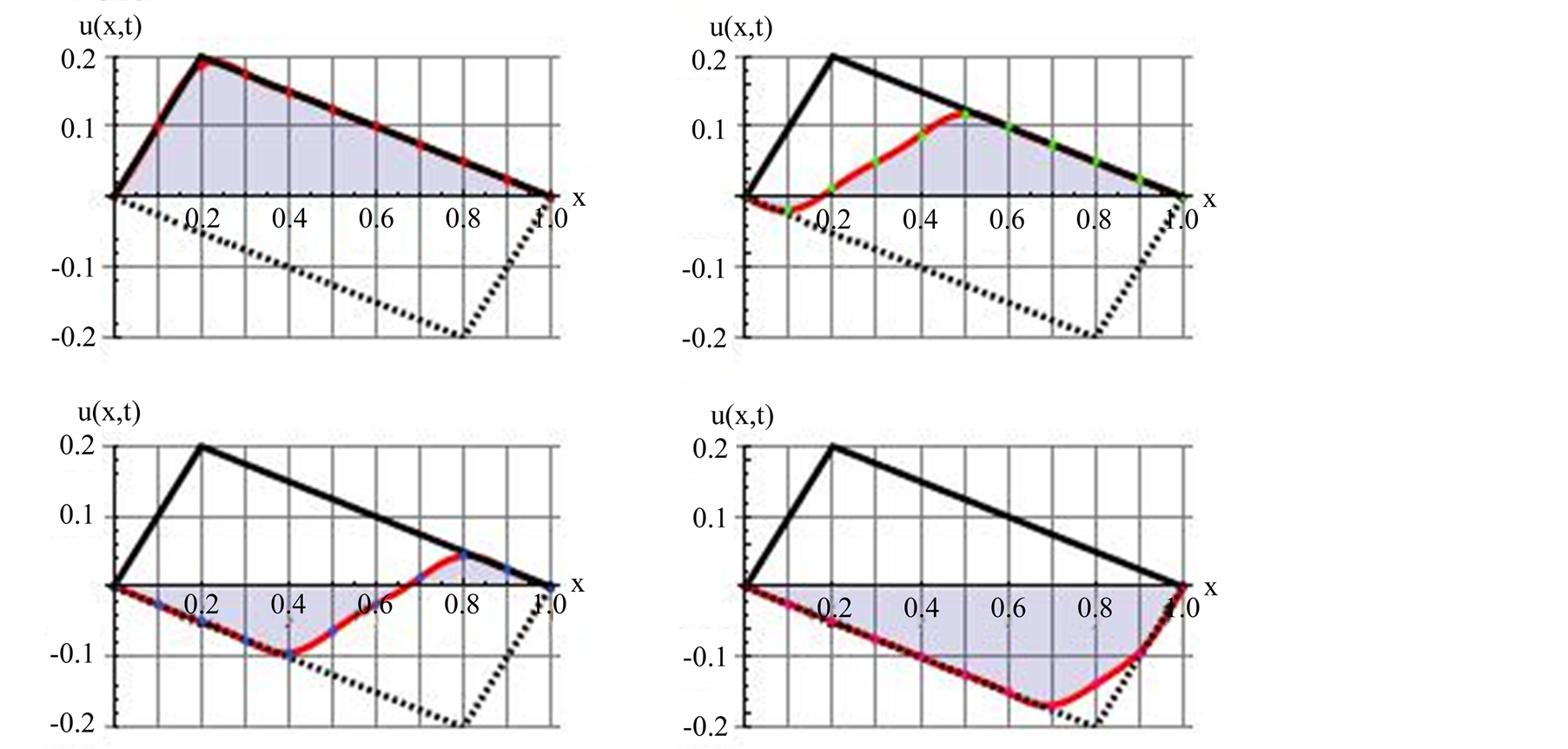
Figure 2. The solid line is the initial profile of the deformed string; the dotted line is its profile at the end of the half of the first cycle. The upper left graph is at t = 0 and the bottom right is at t = 9 s, the other two graphs are for t = 3 and 6 s, respectively.

Figure 3. Graphic description is the same as Figure 2. The difference is the initial deformation is symmetric.
 runs for the case at hand.
3.3. Case 3c
Initial deformation is an asymmetric trapezoid. As we pointed out this is a natural extension of the previous aforementioned cases. Here one pulls the string upward at two different e.g.  points to the same height forming an asymmetric trapezoid. This case has not been reported in the literature. The initial deformation according to Figure 4 is,
 (15)
(15)
where  and
and  are the abscissas of the upper edges of the trapezoid. Following the steps outlined in Case 3a, analytic integration of the given deformation yields,
 (16)
(16)
For instance, for  ten terms of the sum in (15) yields the four snap shots of the vibration displayed in Figure 4.
3.4. Case 3d
Initial deformation is a symmetric parabola. The initial deformation is given by,  , where
  is the maximum height at the mid-point of the line. Utilizing
  and following steps explained in Case 3(a,b& c), the amplitude coefficients evaluate,
  yielding,
 (17)
(17)
Plots of (17) at four different instances are shown in Figure 5. As in the previous cases only a limited number of terms are included in (17).
3.5. Case 3e
Thus far we consider cases where the amplitude coefficients for the chosen initial deformations were analytic. Here we present a case deviating from the norm. Consider an initial deformation such as a symmetric half an ellipse. The deformation is,  , here
  is the height of the mid-point and
  is the line length. Here again the literature search reveals the missed analysis. An attempt was made to calculate the expansion coefficient,
  analytically. We were unable to do so, so did Mathematica. We

Figure 4. Graphic description is the same as Figure 2. The difference is the initial deformation is an asymmetric trapezoid.

Figure 5. Graphic description is the same as Figure 2. The difference is the initial deformation is a symmetric parabola.

Figure 6. Graphic description is the same as Figure 2. The difference is the initial deformation is a symmetric half an ellipse.
then evaluate the integrals numerically. Practically, there are a large number of similar cases, so solving this problem paves the road and proves the usefulness of the CAS. The corresponding Mathematica code is given in the Appendix Case 3e. Utilizing the code four instances of the vibrations are shown in Figure 6.
These snap shots and the corresponding simulation highlight the usefulness of the CAS. Without this simulation one couldn’t envision the intermediate deformations specially the ones shown in the upper right and the lower left of Figure 6.
4. Conclusion
In the first segment of this work, we show the equality of the two seeming different schools of thought concerning the formation of the transverse standing waves. In the second section based on the initial string’s deformations, we examine five cases. The first four are conducive to analytic output, and the fifth requires numeric analysis. We show for both classes of examples how the CAS, especially Mathematica plays an indispensable role. Simulating the vibrations adds a useful dimension to the understanding of the problem. For the interested reader, we have given the Mathematica codes. On the need basses and with minor tweaks, one may also apply the given codes to analyze vast class of the similar problems.
Acknowledgements
The author acknowledges the referee’s suggestion to include the Mathematica code and introducing the reference [10] .
Appendix
Mathematica codes: These codes give the steps needed to simulate the modes of all cases presented in the text.
Code 3a, b:
The parameters are listed in the values.

The initial deformation for the a symmetric triangle  and its form at the end of the first half of the first cycle are named
  and
and , respectivelyg[x_/;0

Equation of the transverse wave, (11 & 14) is,

For eye balling a set of colored dots are introduced.
dots[t_]:=Graphics[Table[{Hue[0.1 t],Disk[{ x,u[x,t]},0.008]},{x,0,{/.values,0.1 {/.values}]]
Simulation of the vibration is given by Manipulate,

A 4 × 4 table displaying snap shots of the vibrations is given bytableu1=Table[Show[{Plot[u[x,t],{x,0, {/.values},PlotRange[{-0.2,0.2},PlotStyle[{Red,Thick},GridLines[{Range[0,1,0.1],Automatic},AxesLabelà{"x","u(x,t)"},FillingàAutomatic],plotinitilpulse,dots[t]}],{t,0,9,3}];
By dropping the semicolon on the next line one gets the Figure 2.
GraphicsGrid[{{tableu1[1\[RightDoubleBracket], tableu1[2\[RightDoubleBracket]},{tableu1[3\[RightDoubleBracket],tableu1[4\[RightDoubleBracket]}}];
Code 3e:
The initial deformation of the symmetric half an ellipse is given by,  , it is named
 .
.

The expansion coefficients are labeled  and their numeric values are,

Utilizing these coefficients we form the wave function.

The rest of the code is the same as Code 3(a, b & c).