Global 1 Estimation of the Cauchy Problem Solutions to the Navier-Stokes Equation

Asset Durmagambetov, Leyla Fazilova

Department Applied Mathematics and Informatics, Buketov Karaganda State University, Karaganda, Kazakhstan.

DOI: 10.4236/am.2014.513184                

Abstract

The analytic properties of the scattering amplitude are discussed, and a representation of the potential is obtained using the scattering amplitude. A uniform time estimation of the Cauchy problem solution for the Navier-Stokes equations is provided. The paper also describes the time blowup of classical solutions for the Navier-Stokes equations by the smoothness assumption.

 

Keywords

Schrödinger’s Equation, Potential, Scattering Amplitude, Cauchy Problem, Navier-Stokes Equations, Fourier Transform, Global Solvability and Uniqueness of the Cauchy Problem, Loss of Smoothness

1. Introduction

In this paper, we introduce important explanatory results presented in a previous study in [1] . We therefore restate the basic to clarify out understanding of them. We begin by considering some ideas about the potential in the inverse scattering problem, and this is then used to estimate solutions of the Cauchy problem for the Navier- Stokes equations. A similar approach has been developed for one-dimensional nonlinear equations [2] - [5] , but to date, there have been no results for the inverse scattering problem for three-dimensional nonlinear equations. This is primarily through difficulties in solving the three-dimensional inverse scattering problem. This paper is organized as follows: the study begin describing the inverse scattering problem, giving in a formula for the scattering potential. Using this potential, we obtain uniform time estimates in time for solutions to the Navier-Stokes equations, which suggest the global solvability of the Cauchy problem for the Navier-Stokes equations. Essentially, the present study expands the results for one-dimensional nonlinear equations with inverse scattering methods to multi-dimensional cases. Our main achievement is a relatively unchanged projection onto the space of solutions associated with the continuous spectrum for the nonlinear equations, which allows us to focus solely on the behavior associated with the decomposition of the solutions to the discrete spectrum. In the absence of a discrete spectrum, we obtain estimations for the maximum potential in the weaker norms, compared with the norms for the Sobolev spaces.

Consider the operators 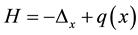and defined in the dense set in the space; let q be a bounded fast-decreasing function. The operator is called the Schrödinger operator. We consider the three-dimensional inverse scattering problem for the Schrödinger operator, i.e, the scattering potential must be reconstructed from the scattering amplitude. This problem has been studied by many researchers ( [6] - [9] , and references therein).

2. Results

Consider Schrödinger’s equation:

. (1)

Let be a solution of (1) with the following asymptotic behavior:

(2)

where is the scattering amplitude and for

(3)

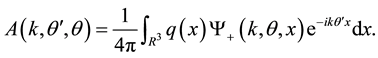
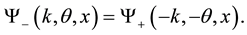
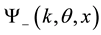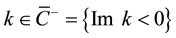Let us also define the solution for as

As is well known [2] :

(4)

This equation is the key to solving the inverse scattering problem, and was first used by Newton [7] [8] and Somersalo et al. [9] .

Equation (4) is equivalent to the following:

(5)

where S is a scattering operator with kernel,

The following theorem was stated in [6] :

Theorem 1. (The energy and momentum conservation laws) Let. Then, , where is a unitary operator.

Definition 1. The set of measurable functions with norm defined by

is recognized as being of Rollnik class.

As shown in [10] , is an orthonormal system of H eigenfunctions for the continuous spectrum. In addition to the continuous spectrum, there is a nite number of H negative eigenvalues, designated as with corresponding normalized eigenfunctions

where.

We present Povzner’s results [10] below:

Theorem 2. (Completeness) For both an arbitrary and for H eigenfunctions, Parseval’s identity is valid.

(6)

where and are Fourier coefficients for the continuous and discrete cases.

Theorem 3. (Birman-Schwinger estimation). Let. Then, the number of discrete eigenvalues can be estimated as:

(7)

This theorem was proved in [11] .

Let us introduce the following notation:

For

(8)

(9)

where

We define the operators for as follows:

(10)

(11)

(12)

Consider the Riemann problem of finding a function, that is analytic in the complex plane with a cut along the real axis. Values of on the upper and lower sides of the cut are denoted and respectively. The following presents the results of [12] :

Lemma 1.

(13)

Theorem 4. Let,; then

(14)

The proof of the above follows from the classic results for the Riemann problem.

Lemma 2. Let Then,

(15)

The proof of the above follows from the definitions of and.

Definition 2. Denote by the set of functions with the norm

Definition 3. Denote by the set of functions such that, for any.

Lemma 3. Suppose. Then, the operator, defined on the set has an inverse defined on.

The proof of the above follows from the definitions of and the conditions of Lemma 3.

Lemma 4. Let, and assume that exists. Then,

(16)

(17)

(18)

The proof of the above follows from the definitions of and Equation (4).

Lemma 5. Let, and assume that exists. Then,

where represents the terms of higher order appearing in.

Proof: Using

and

We establish the proof.

Lemma 6. Let. Then,

(19)

Lemma 7. Let, and assume that exists. Then,

(20)

The proof of the above follows from the definitions of, and Lemma 4.

Lemma 8. Let. Then.

The proof of the above follows from the definition of and the unitary nature of.

Lemma 9. Let. Then,

(21)

(22)

The proof of the above follows from the definitions of, and (1).

Lemma 10. Let. Then,

(23)

The proof of the above follows from the definition of.

Lemma 11. Let, and. Then,

(24)

To prove this result, one calculates

(25)

Using Lemma 5, the first approximation can be obtained in terms of:

(26)

(27)

where represents terms of higher order for and. The lemma can be proved using obvious estimations for and Lemmas 5, 6, and 8.

3. Conclusions for the Three-Dimensional Inverse Scattering Problem

This study has shown once again the outstanding properties of the scattering operator, which, in combination with the analytical properties of the wave function, enable an almost-explicit formula for the potential to be obtained from the scattering amplitude. Furthermore, this approach overcomes the problem of over-determination, resulting from the fact that the potential is a function of three variables, whereas the amplitude is a function of five variables. We have shown that it is sufficient to average the scattering amplitude to eliminate the two extra variables.

4. Cauchy Problem for the Navier-Stokes Equation

Numerous studies of the Navier-Stokes equations have been devoted to the problem of the smoothness of its solutions. A good overview of these studies is given in [13] -[17] . The spatial differentiability of the solutions is an important factor, this controls their evolution. Obviously, differentiable solutions do not provide an effective description of turbulence. Nevertheless, the global solvability and differentiability of the solutions has not been proven, and therefore the problem of describing turbulence remains open. It is interesting to study the properties of the Fourier transform of solutions of the Navier-Stokes equations. Of particular interest is how they can be used in the description of turbulence, and whether they are differentiable. The differentiability of such Fourier transforms appears to be related to the appearance or disappearance of resonance, as this implies the absence of large energy flows from small to large harmonics, which in turn precludes the appearance of turbulence.

Thus, obtaining uniform global estimations of the Fourier transform of solutions of the Navier-Stokes equations means that the principle modeling of complex flows and related calculations will be based on the Fourier transform method. The authors are continuing to research these issues in relation to a numerical weather prediction model; this paper provides a theoretical justification for this approach. Consider the Cauchy problem for the Navier-Stokes equations:

(28)

(29)

in the domain, where:

(30)

The problem defined by (28), (29), (30) has at least one weak solution in the so-called Leray-Hopf class [13] .

The following results have been proved [14] :

Theorem 5. If

(31)

there is a single generalized solution of (28), (29), (30) in the domain, , satisfying the following conditions:

(32)

Note that depends on and.

Lemma 12. Let. Then,

(33)

Our goal is to provide global estimations for the Fourier transforms of the derivatives of the solutions to the Navier-Stokes Equations (28), (29), (30) without requiring the initial velocity and force to be small. We obtain the following uniform time estimation. Using the notation

(34)

(35)

Assertion 1. The solution of (28) (30) according to Theorem 5 satisfies:

(36)

where

This follows from the definition of the Fourier transform and the theory of linear differential equations.

Assertion 2.The solution of (28) (30) satisfies:

(37)

and the following estimations:

(38)

(39)

This expression for is obtained using and the Fourier transform. The estimations follow from this representation.

Lemma 13. The solution of (28), (29), (30) in Theorem 5 satisfies the following inequalities:

(40)

(41)

or

(42)

(43)

This follows from the Navier-Stokes equations, our first a priori estimation (Lemma 1), and Lemma 2.

Lemma 14. The solution of (28) (30) satisfies the following inequalities:

(44)

(45)

(46)

These estimations follow from (9), Parseval’s identity, the Cauchy-Schwarz inequality, and Lemma 3.

Lemma 15. The solution of (28) (30) according to Theorem 5 satisfies, where:

(47)

This follows from our a priori estimation (Lemma 1) and the assertion of Lemma 3.

Lemma 16. The solution of (28) (30) according to Theorem 5 satisfies to the following inequalities:

(48)

where

(49)

Proof. From (36), we have the inequality:

(50)

where

(51)

Using the notation

(52)

And Hölder’s inequality in, the following inequality can be obtained:

(53)

where and satisfy. Let; then

(54)

Using the estimation for in (53), the assertion in the lemma can be proved.

Lemma 17. Let and

Then,

(55)

A proof of this lemma can be obtained using Plancherel’s theorem. For

consider the transformation of the Navier-Stokes:

(56)

Lemma 18. Let

then

Proof. Using the definitions for and we get

(57)

(58)

We now obtain uniform time estimations for Rollnik’s norms of the solutions of (28) (30). The following (and main) goal is to obtain the same estimations for

the velocity components of the Cauchy problem for the Navier-Stokes equations. We shall use Lemmas 6 and 11.

Theorem 6. Let

Then, there exists a unique generalized solution of (28) (30) satisfying the following inequality:

where the value of depends only on the conditions of the theorem.

Proof. It suffices to obtain uniform estimates of the maximum velocity components, which obviously follow from

Because uniform estimates allow us to extend the local existence and uniqueness theorem over the interval in which they are valid. To estimate the velocity components, Lemma 10 can be used:

Using Lemmas (13)-(17) for

we can obtain where is the amplitude of potential and. That is, discrete solutions are not significant in proving the theorem, so its assertion follows the conditions of Theorem 6, which defines uniform time estimations for the maximum values of the velocity components.

Theorem 6 asserts the global solvability and uniqueness of the Cauchy problem for the Navier-Stokes equations.

Theorem 7. Let

(59)

Then, there exists and such that

(60)

Proof. A proof of this lemma can be obtained using and uniform estimates.

Theorem 7 describes the blowup of classical solutions for the Navier-Stokes equations.

5. Conclusion

Uniform global estimations of the Fourier transform of solutions of the Navier-Stokes equations indicate that the principle modeling of complex flows and related calculations can be based on the Fourier transform method. In terms of the Fourier transform, under both smooth initial conditions and right-hand sides, no apparent fluctuations appear in the speed and pressure modes. A loss of smoothness in terms of the Fourier transform can only be expected for singular initial conditions or unbounded forces in. Theorem 7 describes the time blowup of the classical solutions for the Navier-Stokes equations arises, and complements the results of Terence Tao [17] .

Acknowledgements

We are grateful to the Ministry of Education and Science of the Republic of Kazakhstan for a grant, and to the System Research “Factor” Company for joint efforts in this project. The work was performed as part of an international project, “Joint Kazakh-Indian studies of the influence of anthropogenic factors on atmospheric phenomena on the basis of numerical weather prediction models WRF (Weather Research and Forecasting)”, commissioned by the Ministry of Education and Science of the Republic of Kazakhstan.

Conflicts of Interest

The authors declare no conflicts of interest.

References

[1]	Durmagambetov, A.A. and Fazilova, L.S. (2014) Global Estimation of the Cauchy Problem Solutions’ the Navier-Stokes Equation. Journal of Applied Mathematics and Physics, 2, 17-25. http://dx.doi.org/10.4236/jamp.2014.24003
[2]	Russell, J.S. (1844) Report on Wave. Report of the 14th Meeting of the British Association for the Advancement of Science, York, September 1844 (London 1845), Plates XLVII-LVII, 90-311.
[3]	Russell, J.S. (1838) Report of the Committee on Waves. Report of the 7th Meeting of British Association for the Advancement of Science, John Murray, London, 417-496.
[4]	Ablowitz, M.J. and Segur, H. (1981) Solitons and the Inverse Scattering Transform SIAM, 435-436.
[5]	Zabusky, N.J. and Kruskal, M.D. (1965) Interaction of Solitons in a Collisionless Plasma and the Recurrence of Initial States. Physical Review Letters, 15, 240-243. http://dx.doi.org/10.1103/PhysRevLett.15.240
[6]	Faddeev, L.D. (1974) The Inverse Problem in the Quantum Theory of Scattering. II. Itogi Nauki i Tekhniki. Ser. Sovrem. Probl. Mat., VINITI, Moscow, 93, 180.
[7]	Newton, R.G. (1979) New Result on the Inverse Scattering Problem in Three Dimensions. Physical Review Letters, 43, 541-542. http://dx.doi.org/10.1103/PhysRevLett.43.541
[8]	Newton, R.G. (1980) Inverse Scattering in Three Dimensions. Journal of Mathematical Physics, 21, 1698-1715. http://dx.doi.org/10.1063/1.524637
[9]	Somersalo, E., et al. (1988) Inverse Scattering Problem for the Schrodinger’s Equation in Three Dimensions: Connections between Exact and Approximate Methods. http://conservancy.umn.edu/bitstream/4896/1/449.pdf
[10]	Povzner, A.Y. (1953) On the Expansion of Arbitrary Functions in Characteristic Functions of the Operator . Russian Matematicheskii Sbornik, 32, 109.
[11]	Birman, M.S. (1961) On the Spectrum of Singular Boundary-Value Problems. Russian Matematicheskii Sbornik, 55, 125.
[12]	Poincare, H. (1910) Lecons de mecanique celeste. t. 3, 347-349.
[13]	Leray, J. (1934) Sur le mouvement d’un liquide visqueux emplissant l'espace. Acta Mathematica, 63, 193-248. http://dx.doi.org/10.1007/BF02547354
[14]	Ladyzhenskaya, O.A. (1970) Mathematics Problems of Viscous Incondensable Liquid Dynamics. M:Science, 288.
[15]	Solonnikov, V.A. (1964) Estimates Solving Nonstationary Linearized Systems of Navier-Stokes’ Equations. Transactions Academy of Sciences USSR, 70, 213-317.
[16]	Huang, X.D. and Li, J. and Wang, Y. (2013) Serrin-Type Blowup Criterion forFull Compressible Navier-Stokes System. Archive for Rational Mechanics and Analysis, 207, 303-316. http://dx.doi.org/10.1007/s00205-012-0577-5
[17]	Terence Tao (2014) Finite Time Blowup for an Averaged Three-Dimensional Navier-Stokes Equation. arXiv:1402. 0290 [math. AP]