Measurements of the Thermophysical Properties of the API 5L X80 ()
1. Introduction
The correlation between microstructure and mechanical properties in high strength low alloy (HSLA) steels has been analyzed by many researchers [1] [2] . However, the thermophysical properties of these microalloyed steels have been little studied.
In recent years, in order to increase product quality and reduce cost, the industry has placed more and more emphasis on advanced numerical simulation technology to better understand the critical parts of the thermal evolution, stress and microstructure during welding, casting and other manufacturing processes [3] . Although the numerical models are quite advanced and have a high potential for improving the quality of products, leading to a better understanding of materials behavior, their success depends, in large part, on an accurate thermophysical property database. However, the required input data of thermophysical properties necessary for accurate simulations are frequently nonexistents or unreliables at elevated temperature [3] -[5] for many alloys of interest for engineering. Considering the improved performance of computers with a cost relatively low, threedimensional modeling become an attractive possibility for the design and optimization of welded structures with respect to the residual stresses and deformations [5] .
Several approaches of two-dimensional analysis have been performed using well known materials. However, in many cases, a two-dimensional model is not suitable. The “nature” of the welding process often requires a three-dimensional analysis [3] -[7] . These models may include non-linearities in the material such as thermophysical properties (thermal conductivity, specific heat, thermal expansion coefficient, etc.), all temperature dependent. It is also necessary to consider the complex of thermal and mechanical contours conditions and latent heat [4] . The distribution of the heat coming from the fusion zone to the base metal results in high temperature gradients, which also produces considerable variations in the mechanical properties of the material [7] -[9] .
In the analysis of heat transfer problems, it is necessary to know the various thermophysical properties of matter, which are divided into two distinct categories [10] : the transport properties and the thermodynamic properties. The transport properties including diffusion coefficients rate as the thermal conductivity , which represents the ease with which the heat conduction in the material, being defined by Fourier’s law (Equation (1))
 (1)
(1)
where  is the heat flux in the
  direction and
  is the temperature gradient in the same direction. Similar definitions are associated with other directions, but in an isotropic material the thermal conductivity is independent of direction.
Richter [11] and Powell [12] have reported physical properties as a function of temperature for a number of different steels. The thermal conductivity of steel alloys diverges when temperature is decreased. The pure iron having the highest thermal conductivity is followed by carbon steels, alloy steels and then by high-alloy steels. High-alloy steels have lower thermal conductivity at ambient temperatures than at high temperatures. At higher temperatures, in austenite domain, all the alloys have similar thermal conductivities.
In addition to the transport properties, there are thermodynamic properties, which are related to the equilibrium state of a system. Two of these properties widely used in heat transfer analysis are the density  and specific heat
 . The product
  [J/m3∙K], called volumetric heat capacity, is the ability of a material to store thermal energy [10] .
The ratio between the thermal conductivity and volumetric heat capacity is called thermal diffusivity. This is an important property that measures the ability of a material to conduct thermal energy relative to its ability to store it, and thus the response speed of the material in relation to changes in thermal conditions [10] .
The specific heat is understood as the amount of heat needed to change one degree in the temperature of a unit mass. This property is crucial to determine the amount of energy to be added or removed in the processes of heating and cooling [10] .
2. Material and Methods
The material used in this work was the API 5L X80 steel with a thickness of 19 mm. This steel with wide application in the oil and gas has a chemical composition shown in Table1
The thermal expansion coefficient , specific heat
 , thermal diffusivity
  and thermal conductivity
  of API 5L X80 steel were experimentally measured as a function of temperature.

Table 1. Chemical composition of API 5L X80 steel (% mass).
2.1. Thermal Expansion Coefficient
To obtain the thermal expansion coefficient of API 5L X80 steel, dilatometry tests were carried out in a DIL 402 PC dilatometer.
For these tests, cylindrical specimens with 5 mm of diameter and 25 mm of length were manufactured from API 5L X80 steel. These samples were subjected to heating and cooling steps, in order to obtain the phase transformation temperatures of the steel and the thermal expansion coefficient of the material with temperature.
The DIL 402 PC dilatometer has the following technical specifications:
Ø temperature range: from room temperature to 1200˚C;
Ø heating rates: 0.01 K/min to 50 K/min;
Ø measuring range: 500 μm/5000 μm;
Ø sample length: 50 mm (máx.);
Ø sample diameter: 12 mm (máx.);
Ø resolution : 8 nm.
2.2. Specific Heat
The measurement of the specific heat of API 5L X80 steel was carried out in the Differential Scanning Calorimetry (DSC)/Differential Thermal Analysis (DTA)-LABSYS evo.
The specific heat  of a sample is defined as:
 . Three different methods can be used for the determination of specific heat: the continuous, the stepwise and the drop methods. The first two methods can be used for
  determination of solids and liquids. The drop method can be only used for solids.
The stepwise method gives usually a better result, but takes more time to implement. In this study stepwise method was used to measure the specific heat.
To make quantitative measurements the  sensor needs to be calibrated. The calibration has been done using sapphire α-Al2O3 as standard because data on this material are easily available in the literature. Thus, the procedure for measuring the specific heat of a material sample follows 3 steps:
1) Measurement of a blank;
2) Measurement of a calibration reference (sapphire standard);
3) Measurement of the sample.
The calculation is the carried out in the processing section of the software using the following equation (Equation (2)):
 (2)
(2)
In this equation,  and
and  are the amplitudes of the blank, of the sample and of the calibrant respectively, all measured in
 . The
. The  and
and  are the weights of the calibrant and the sample respectively, and
  is the specific heat of calibrant.
For temperatures from 70˚C to 1600˚C the specific heat of the calibrant is represented by the following polynomial function (Equation (3)):
 (3)
(3)
In this equation,  and
and  is the temperature.
2.3. Diffusivity and Thermal Conductivity
In order to obtain the diffusivity and thermal conductivity of API 5L X80 steel a technique called laser flash was used in a Micro Flash LFA 457 diffusivimeter. The LFA 457 is an instrument used to measure these properties in metals, graphite, coatings, composites, ceramics, polymers, liquids and other materials.
The Flash method is used in 80% of the measured thermal diffusivity across the world and became an ASTM standard (ASTM 1461-01, 2001) [13] . When compared with the direct measurement of thermal conductivity, the advantages of this method are:
Ø Sample geometrically simple, small size and easy to prepare;
Ø Applicability to a wide range of diffusivity values of 0.001 cm2/s to 10 cm2/s and temperatures from −125˚C to 1100˚C;
Ø Excellent accuracy;
Ø A wide temperature range can be covered in a short period of time when a little time is required for a single measurement.
The sample is mounted in the system support which is located inside the furnace. While the sample reaches a predetermined temperature, the energy supplied by a laser pulse is absorbed by the bottom face of the sample, resulting in heating of this. The heat propagates through the sample by conduction, increasing the temperature of the upper surface. The temperature rise is measured on this face as a function of time by an infrared detector. The thermal diffusivity is calculated by the software, through mathematical models selected.
The vertical construction of the measuring unit is the primary component of the system. The laser system is mounted in a closed wrapper at the bottom. A receiver block is located above the laser system. The cylindrical sample holder (Figure 1) and its regulating device are mounted on this block. A seal enables a vacuum, or the existence of a controlled atmosphere within the furnace. The system of the furnace is raised and lowered by a mechanical jack. The laser is emitted with a wavelength in the infrared band with 1064 nm, while the pulse width is variable. A thermocouple is placed at the side of the sample carrier tube, serving to measure the temperature inside the oven and therefore the samples. Different thermocouples may be used depending only on the temperature range of interest, and using a liquid nitrogen tank as a reference value, the infrared detector measures the temperature rise on the upper surface of the sample.
The samples used in this experiment were cylindrical with a diameter of 12.5 mm and a thickness of 3 mm. The faces of these samples were coated with a graphite special ink of black color, in order to increase either the surface absorptivity, improving the absorption of the energy pulse, or the emissivity, enhancing the emission of radiation and reading the IR sensor.
At the end of the test, the results are analyzed in PROTEUS software. Here, the heating curve of each pulse can be viewed individually as well as the test conditions. The mathematical model can be chosen from among the existing or fail to choose the by software, admitting that it select the one that best matches the heating curve at each point.
3. Results and Discussion
The theoretical works on heat transfer in the welding process began with Rosenthal in the 40’s [14] [15] . However analytical solutions of the thermal problem for welding were obtained with some simplifications, among them, the variation of thermophysical properties with temperature is neglected so the average values were adopted. Obviously, various physical properties of the material such as its thermal conductivity vary with temperature. Taking into account this variation, the problem becomes very complex or impossible, so that the analytical solution requires the use of a numerical method.
3.1. Thermal Expansion Coefficient
The dilatometry is one of the most powerful techniques for the study of phase transformations in solid state, because it allows the monitoring of the evolution of changes in real time in terms of dimensional changes that occur in the sample by applying athermal cycle. The applicability of dilatometry in research of phase transformation is due to the change of the specific volume of a sample during a phase transformation. When a material undergoes a phase transformation, the crystal structure changes and this is normally accompanied by a change in specific volume [16] .
A graph of dilatometry as a function of temperature and time concerning a dilatometric test was carried out on API 5L X80 steel in the condition of “as received” (Figure 2).
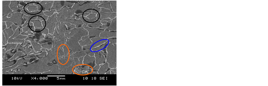
The microstructure of the material “as received” was observed by Scanning Electron Microscopy (SEM) and

Figure 2. Measured results of the thermal expansion coefficient [K−1] of the API 5L X80 steel.
is shown in Figure 3, with increases of 4000 and 10,000X, which allowed us to characterize the constituent phases. In these micrographs, the microstructures are predominantly formed by polygonal ferrite (black ellipses). The whitish grain boundaries characterizing a solute enrichment at the grain boundaries (blue ellipses) also been observed. In addition, it is also possible to observe the presence of perlite (orange ellipses) in some grain boundaries.
In the dilatometric test, the material was heated with a heating rate of 10˚C/min until a temperature of 950˚C and then it was maintained at this temperature for 10 minutes to ensure complete austenitizing, and finally it was cooled with a cooling rate 5˚C/min to the temperature of 300˚C (red curve, Figure 2). In addition to obtaining the phase transformation temperature of the steel during thermal cycling (white curve, Figure 2), the dilatometric technique can also be used for measuring the thermal expansion coefficient of this material as a function of temperature (blue curve, Figure 2).
During the heating step, the thermal expansion coefficient of the steel remains approximately constant with a value of , however, the thermal expansion coefficient is dropped reaching a minimum of approx-
 (a)
(a) (b)
(b)
Figure 3. SEM micrographs of API 5L X80 steel in condition as received. (a) 4000X and (b) 10,000X.
imately  at temperature of 890˚C, due to the occurrence of the phase transformation
  in the temperature range of 730˚C to 890˚C. At the end of this transformation, the thermal expansion coefficient becomes to the value of
 .
.
During the cooling step, the thermal expansion coefficient of the steel remains approximately constant with a value of , however, the thermal expansion coefficient undergoes another drop reaching a minimum of approximately
  at temperature of 685˚C, due to the occurrence of the phase transformation
  in the temperature range of 785˚C to 685˚C. At the end of this transformation, the thermal expansion coefficient becomes to the value of
 .
.
It is clearly shown that between the heating step and cooling step has a region of disturbance in the behavior of the thermal expansion coefficient of the steel (higher peaks). The reasons for this may be also associated to phase transformations (austenite decomposition), which may have occurred during the isothermal stage 950˚C.
3.2. Specific Heat
The measured results of the specific heat are shown in the graph below (Figure 4). In this work, values of specific heat of API 5L X80 steel have been measured in the range 300˚C to 1200˚C with a step  of
of . It is observed (Figure 4) for this material, in the considered range, minimum and maximum values of specific heat equal to 0.571 J/gK and 1.084 J/gK at temperatures of 300˚C and 720˚C, respectively. According to Pedrosa [17] , this peak that appears in the curves
  versus
  and
and  versus
 , is due to the occurrence of phase transformation
  in steel. It is clearly observed that the peak present at the
  versus
  curve (Figure 4) shows a maximum value of
  equal to 1.084 J/gK at 720˚C and then drops to 0.603 J/gK at 880˚C. This behavior shows the occurrence of the phase transformation
  in this temperature range, being in agreement with the dilatometric curve (Figure 2).
Li [3] , studying the thermophysical properties of the AISI 4320 and 4130 steels found the same behavior of the  versus
  curve. The curve has a significant endothermic peak starting around 700˚C. This peak represents the solid state austenite phase transformation and extends to around 825˚C. A similar behavior of
  versus
  curve is also found for pure iron (Figure 5). Here the peak starting at around 725˚C and extends to around 925˚C.
A similar behavior of the curve  versus
  but with different values of specific heat was obtained [18] in a low carbon steel (0.1% C). The same happened with Deng [19] studying two carbon steel of 0.15% C and 0.45% C.
Attarha and Sattari-Far [20] , studying a carbon steel with 0.15% C, found results similar to those obtained in this work until the temperature of 400˚C. Above 400˚C their results were very different with a maximum value to the specific heat equal of 0.863 J/gK to 1300˚C.Very different results were found by Shan [21] , who used these properties in a stainless steel which is not transformed in the temperature range of our study.
3.3. Thermal Diffusivity and Thermal Conductivity
For all measurements, the software PROTEUS showed that the model that best represented the data obtained in
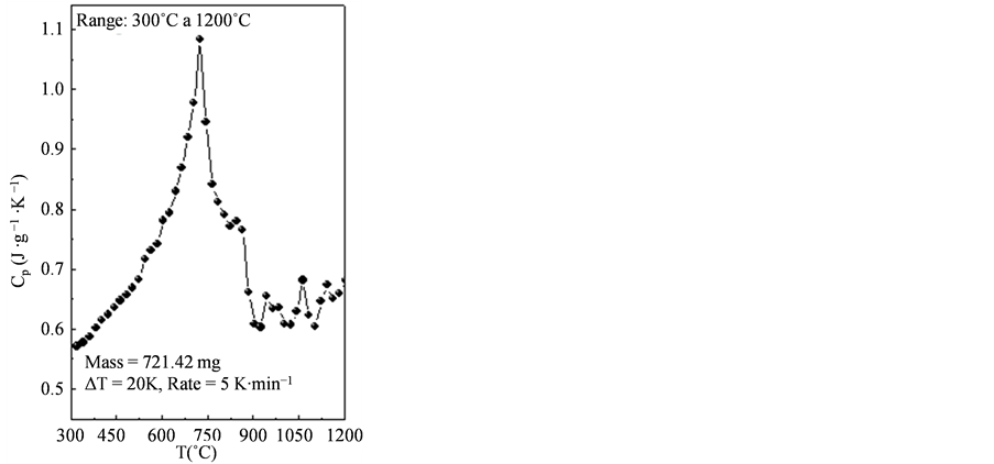
Figure 4. Measured results of the specific heat [J/gK] of the API 5L X80 steel.
 (a)
(a) (b)
(b)
Figure 5. Measured results of the specific heat [J/gK] a) in the pure iron and b) in the AISI 4130 and 4320 steels, adapted from [3] .
this study was the Cape and Lehman model with correction pulse. The mathematical model of Cape and Lehman [22] is more complex than that of Parker [23] , and use more complex and comprehensive considerations:
Ø Two-dimensional conduction with symmetry in respect to the central axis;
Ø The energy absorbed by the sample as a source-term in the energy equation;
Ø Uniform energy flow, completely absorbed at ;
;
Ø Losses heat surfaces taken into account as a linearized radiation term.
Using a sample of thickness  and radius
 , originally at temperature
 , the model is given by (Equation (4)):
 (4)
(4)
where: 
 (5)
(5)
In Equation (5),  is the Stefan-Boltzmann constant (
 W/m2K4) and ε is the emissivity of the surface.
The graphics generated by the diffusivity and thermal conductivity were calculated by software based on each pulse done on the samples (Figure 6). Through these, it can be seen that any point may have any inadequacy in the result of measurement.
In this work, the diffusivity and thermal conductivity values of API 5L X80 steel were measured in the range 100˚C to 800˚C with a step  50
50 . It is observed (Figure 6) within the range considered that this material has minimum and maximum values of diffusivity equal to 3 J/gK, and 13 J/gK at temperatures of 750˚C and 100˚C, respectively. The thermal conductivity also shows minimum and maximum values equal to 13 W/mK and 52 W/mK at the same temperatures. It is clearly shown that two of the points obtained at a temperature of 500˚C does not fit the trend of the points and should be disregarded. The reasons for this may due to fluctuations in the mains voltage, which may have interfered with the signals from the various instruments in operation. A similar behavior
  versus
  curve is also found for pure iron (Figure 7).

Figure 6. Measuments of the thermal diffusivity [mm2/s] and thermal conductivity [W/mK] of theAPI 5L X80 steel.

Figure 7. Obtained results of the thermal conductivity [W/mK] of the pure iron.
Deng [19] obtained a similar behavior  versus
  curve, but with different values of thermal conductivity, studying a steel with carbon content of 0.15% C and 0.45% C. The same behavior in the
  versus
  curve was also observed in the work of Tsirkas [24] in the AH 36 steel. Different results were found by Klobcar [25] studying the temperature distribution generated by GTAW welding in a H13 steel. The same occurred with Dhingra and Murphy [26] studying the temperature distribution generated by GMAW welding in a butt joint of a low carbon steel.
According to Deng [19] , one must consider the effects of the flow of liquid metal on the temperature distribution in a welded joint. If this effect is neglected in the modeling, a higher temperature value will be obtained in the weld pool. Using the dual-ellipsoidal source model of Goldak [27] [28] , one value above 3000˚C can be obtained, thus very different from realistic situation. To avoid these problems in their study, Deng saw an increase in thermal conductivity to offset the effect of the flow of liquid metal in the weld pool. When the temperature is higher than the melting point, the thermal conductivity value is assumed to be approximately two times higher than that at room temperature.
Peet [29] predicted the thermal conductivity of steels had a strong significance in the behavior if the manganese, nickel, molybdenum and chromium were present. Carbon, silicon, vanadium and copper had a lower significance, while elements titanium, tungsten, niobium and aluminium had very low significance. Following these authors [29] , the aluminum, with lowest significance, is a strong carbide forming, as such it may usually form second phases not affecting the thermal conductivity greatly, except by removal of carbon or nitrogen.
The numerical finite element method (FEM) can predict the temperature field along the welded component. A challenging part to provide precise numerical results is the experimental measurement of the thermophysical properties of the material, thereby causing behavior of the modeled component reflects the real behavior. If, in the numerical simulation, this set of properties is available and the generated mesh has refinement sufficient, the temperature distribution due to welding can be obtained accurately along the model, making the finite element method highly effective. The use of thermo-physical properties not belonging to the material studied provides erroneous numerical results.
● 4. Conclusions
● The dilatometric test carried out in the API 5L X80 steel showed the occurrence of phase transformations  and
and  during heating and cooling steps in the temperature ranges from 730˚C to 890˚C and 785˚C to 685˚C, respectively. The thermal expansion coefficient remained approximately with constant value of
 , however, due to the occurrence of these phase transformations during the stages of heating and cooling, the thermal expansion coefficient of steel suffer two falls reaching values
  and
and , respectively. At the end of these transformations, the thermal expansion coefficient becomes to the value of
 .
.
● It is observed that this material, in the temperature range 300˚C to 1200˚C, shows minimum and maximum values of specific heat equal to 0.571 J/gK and 1.084 J/gK at temperatures of 300˚C and 720˚C, respectively. The presence of this peak in the curve , shows the occurrence of phase transformation
  in the steel.
● The behavior of thermal diffusivity and thermal conductivity of API 5L X80 steel, in the temperature range 100˚C to 800˚C, tends to decrease with increasing temperature, with minimum and maximum values of diffusivity equal to 3 J/gK, and 13 J/gK at temperatures of 750˚C and 100˚C, respectively, and thermal conductivity equal to 13 W/mK and 52 W/mK at the same temperatures.
Acknowledgements
We’d like to thank Calorimetry Laboratory of the Department of Physics of Pernambuco Federal University for the DSC tests, as well as to Solar Energy Laboratory of Paraiba Federal University for the laser flash tests. We also thank the CONFAB for providing the material of this study.
NOTES
*Corresponding author.