Nonlinear Model of Image Noise: An Application on Computed Tomography including Beam Hardening and Image Processing Algorithms ()
1. Introduction
Noise is considered a critical factor in Computed Tomography (CT) because it establishes an inferior limit to the contrast detectable by the observer. The collective dose is increasing worldwide due to CT examinations and its reduction which poses an optimization problem: while the lower the dose the higher the image noise. Previous models of image noise had been reported [1] -[4] . For instance, the model of noise in [1] is still useful to understand the association of noise with dose, attenuation, and acquisition parameters in spiral CT, but is incomplete because the image quality is only considered in terms of quantum noise and spatial resolution. Other important influences, which lead to image quality variations, such as beam hardening and reconstruction algorithms implemented by manufacturers can no longer be described by such a simple equation. A correlation between image noise and dose for each examination protocol was determined by measuring the noise while keeping the scanning parameters other than tube current constant in [3] [4] . A more inclusive noise model could provide knowledge about quantitative effect of reconstruction algorithms and beam hardening and a predictive tool for clinical applications. The aim of this work was to model the effect of scanning factors on image noise, including attributes of the scanned object, quantitative and qualitative factors and beam hardening considerations.
The modelling of noise has a great importance from both descriptive and predictive points of view, taking into account its association with the physical quantities involved in the clinical applications of CT.
2. Materials and Methods
The analytical models can be used to quantitatively understand the association between the image quality and operational factors of CT machines and the properties of the scanned object.
2.1. Definition of General Noise Model
According to reported noise models [1] -[4] , the deterministic association between image noise and operational factors can be expressed, in general, by the product of power functions as presented in Equation (1). The noise  depends of multiple quantitative factors: the tube current time product
 , effective attenuation of the scanned object
 , the slice thickness
  and the reconstruction diameter
 . In general, CT users do not know the exact functions of reconstruction modes, algorithms (kernels) and available post-processing tools installed on CT machines, but they can be included as qualitative factors into mathematical models.
In our proposal, the quantitative impact of qualitative factors on noise is expressed in exponential form  of binary variables
  (i > 4). The quantitative effect of image processing factors will be identified through positive coefficients as in [5] , which express their impact on noise reduction, or its increase with values less or greater than unity respectively.
 (1)
(1)
where  is the error term, assumed as a random variable with normal distribution, constant variance and the expected value zero. The parameter of proportionality
  has units of
  and is associated with technological factors of the CT system (for instance, detector’s efficiency, Data Acquisition System and geometrical aspects). The confidence interval and value of
  will depend on which factors are not included as predictors.
In order to find the physical meaning of model parameters, the partial derivatives can be found as in Equation (2), which provide the rate of noise variation (RNVi) with respect to a given .
.
 (2)
(2)
The value of  determines the RNVi associated with the technological factors above mentioned, this means that images from machines of CT with lower values of
  will have lower noise levels, considering there are no significant differences among their corresponding parameters and equivalent levels of physical magnitudes. The RNVi associated with factor
  is explained by each
 , and the RNVi associated with the remaining factors
  is explained by the product of the corresponding power functions for a given level of
 . For factors with
 ,
,  and monotonous increasing when
  increases, favouring lower noise levels, because the power law decreases for a given combination of
 .
.
The tube potential was taken into account for obtaining the experimental design, but is not included as a predictor of the nonlinear noise model because its effect is present in the effective attenuation factor , which depends on the spectrally distributed energy fluence at the entrance of a homogeneous water phantom
  and the fluence
  after the beam traversed the phantom, see Equation (3). The factor
  describes the effective attenuation of photons, considering beam hardening [6] . Due to the dependence of the linear attenuation coefficient with respect to energy, the attenuation does not satisfy the Lambert-Beer law for polychromatic beams. Thus
  is defined as the ratio of spectrally distributed energy fluence at the entrance of a homogeneous water phantom, whose total thickness is L, and the energy fluence at the exit of the same minus one:
 (3)
(3)
where  is the linear attenuation coefficient averaged over the local spectrum of photons at a depth l, considering the effect of polychromatic beam hardening. In general, when
 , the measured in air noise is zero; note that the definition of
  satisfies this technological condition.
The  corresponding to water was estimated according to the methodology developed in [7] . The linear attenuation coefficient of water
  was obtained using the program XMuDat [8] , discretizing the energy range from 1 keV up to 140 keV (steps of 1 keV). The attenuation coefficient was adjusted to Equation (4) according to the energy levels E (MeV) and a given material,
 (4)
(4)
where  are parameters obtained by nonlinear fitting and
  is the Klein-Nishina cross section, which was estimated by Equation (5).
 (5)
(5)
where ,
,  and
and  is the classic electron radius.
For the application of the proposed model a Single Detector Scanner was used (SHIMADZU SCT-7800 TC, Kyoto, Japan). The energy fluence  of the spectrum incident on the phantom was estimated for each tube potential level available (120 and 135 kV) on CT machine, determining incident spectra was performed using the program xcomp5 v.3.5 [9] with an anode angle of 7˚, at a distance of 31 cm from the focal spot and a thickness of absorber of 2.2 mm Al + 1 mm PMMA (Polymethyl Methacrylate), whose characteristics are similar to the tube and cover of the CT machine used for the estimation of the model. The energy fluence at the exit of the scanned object
  was estimated by discretizing the distance l and the energy by steps of 0.1 cm and 1 keV respectively, the integral was numerically calculated by using the trapezoidal method. The averaged linear attenuation coefficient
  was calculated according to the method described in [7] in order to obtain
 . The effective attenuation coefficient
  was obtained for each level of fluence by adjusting the exponential
 , considering beam hardening.
The proposed model presented in Equation (1) includes qualitative factors and beam hardening effect on noise in addition to previous models of image noise [1] -[5] , which therefore represents a more inclusive nonlinear model of noise.
2.2. Experimental Design
Several practical difficulties are presented on the estimation of the model assumed according to Equation (1):
• To estimate the functional part, it requires a set of pixel noise measurements for different combinations of levels of physical factors. One option could be a full factorial design, which would imply overexploitation of the CT unit, for which are necessary more than 80,000 combinations of predictors levels, making very difficult to estimate the model due to this experimental limitation plus associated costs, especially in a machine dedicated to clinical diagnosis. The difficulty lies in determining an experimental design with the necessary combinations of predictor’s levels that satisfy a high prognostic value of the model.
• Furthermore, the estimation of nonlinear models also requires a priori knowledge of a vector of model parameters.
• Nonlinear statistical models such as the one proposed are based on certain assumptions, for example the normal distribution of measurement values. If the probabilistic distribution of error is asymmetric or prone to outliers, the model assumptions would be invalidated and parameter estimates, confidence intervals and other statistics calculated would not be reliable. It is usual to find outliers of measured noise values in images from equipment for clinical use, which are not excludable for estimating the model as part of the experimental space.
To overcome the practical difficulties mentioned and to get the experimental design, a four step methodology was applied:
1) Obtaining an experimental design matrix with the minimum amount of combinations of levels of factors to guarantee an acceptable level of Predicted Error Variance of the model . This is possible through an experimental design of optimal variance (V-optimal design) [10] , which was performed by using the set of tools Model-Based Calibration Toolbox, (MATLAB v.7.6 R2008a, MathWorks Inc.) [10] , available for linear models. Therefore it was necessary to estimate a multiple linear regression model according to Equation (6), where Y corresponds to the logarithm of the noise measured, and the functional part as the logarithm of the nonlinear function given in Equation (1).
 (6)
(6)
where ,
,  is the constant of the linear model and
  (i > 0) are now the parameters of a multiple linear regression model, each
  was estimated for every
 , and for i > 4,
  values corresponds with binary values of qualitative variables,
  is the error term of the linear model, which is assumed here as a random variable of normal distribution with constant variance and expected value is zero.
2) For the experimental design a criterion of  was established, assuming an expected mean square error of
 . The optimal design criterion was established as
 , where G is the maximum value of the prediction error variance of the experimental design
 , which is associated with the
  according to Equation (7).
 (7)
(7)
The levels of  for the design were selected according to those available on the CT machine used and the required transformations for Equation (6). The levels of
  correspond to the natural logarithm of 40, 50, 100250, 400 and 800 mAs respectively. The levels of
  were calculated according to the combinations of each tube potential level (120 and 135 kV) with diameters levels shown in the phantoms Figure 1. These were used to simulate dimensions equivalent to an adult skull, and to the abdomen of paediatric patients, with the intermediate cylinder of 16 cm (PMMA walls), and to an adult abdomen with the largest diameter of 23 cm, shown in Figure 1(a). The neonate skull was simulated with a bottle of 5 cm in diameter as shown in Figure 1(b), with walls of Polyethylene Terephthalate (PET).
The levels for X3 and X4 were estimated as logarithms of the slice thicknesses 0.1, 0.3 and 1 cm and for fields of view (FOV) of 5 and 50 cm respectively.
For qualitative factors, the levels selected were transformed into binary variables for the following reconstruction modes: Standard “STD”, high resolution “HR”, motion compensation “MAC”, reconstruction of two frames per tube rotation “2segs” and reconstruction of three frames per tube rotation “3segs”. The levels of kernel were selected as: “RF1” (Extra smoothing), “RF2” (Smooth), “RF3” (Standard), “RF4” (Fine), “RF5” (Extra Fine) and “RF6” (for evaluation with water phantoms).
The levels of post-processing filters of type “Smart Filter” selected were: “SF1” (Weak), “SF2” (Middle) and “SF3” (Strong) [11] . Binary variables for levels “3segs”, “RF6” and “SF3” were excluded to avoid computational problems leading to linear dependencies between the columns of factors matrix [10] and they were the levels of less practical importance for the proposed model. Some restrictions were imposed to binary variables as reconstruction mode, kernel and Smart Filters as follows: ,
,  and
and  respectively,

Figure 1. Water phantoms: (a) PMMA walls, with central pin in section of 10 cm, middle section (16 cm), and the largest section of 23 cm diameter, (b) PET bottle (5 cm).
because they can only be selected operationally by combining a reconstruction mode with a kernel and a “Smart Filter” simultaneously for each image.
3) Experimental measurements are described in the section Procedure of Experimental Measurements.
4) As it is necessary to have an initial vector of parameters for the nonlinear model, the parameter vector  would serve for this purpose. The parameters were estimated from the linear model given by Equation (1), as explained in the section of Estimating the Linear Model.
It is important to note that the use of  as initial vector for estimating
  should be done with caution, because although the nonlinear function of Equation (1) could be transformed using logarithm, this does not necessarily imply that the linearized model parameters correspond to the nonlinear model, so the use of
  could lead to inadequate physical interpretations. This is because the logarithmic transformation of the nonlinear model will affect the error term in general, so there is no guarantee for the fulfilment of important assumptions for robust nonlinear regression as normality and homoscedasticity of
 .
.
Nonlinear model parameters were estimated by nonlinear robust fitting, which is less sensitive to large changes in small portions of data than the OLS. The method used is explained in the section Method for Estimating the Nonlinear Model.
2.3. Procedure of Experimental Measurements
Before starting the measurements, a calibration was performed to the CT machine to ensure operations in similar conditions to clinical use. Axial images were obtained sequentially according to the combinations of levels obtained in the experimental design. Three replicates were performed for each combination of levels from predictors. The noise was calculated as the standard deviation of the pixel intensities in Hounsfield units (HU), contained in a square region of interest (ROI) in the centre of each axial image.
The number of pixels within the ROI could change the value and variability of , as the experimental design requires different diameters and combinations of levels where in some cases the FOV is smaller than the phantom’s diameter, the ROI size was defined as a percentage of the internal phantom’s diameter for images where the diameter was smaller than the FOV-see Figure 2(a), and a percentage of the FOV if otherwise-see Figure 2(b). The ROI size effect on the nonlinear model was analysed by estimating the variation of parameters and the coefficient of determination according to different ROI sizes (from 10% to 70% of phantom’s diameter or FOV).
The range of scanning time per rotation, tilting and rotation angle were 1 - 3.2 s, 0˚ and 360˚ respectively. The phantoms were placed using the laser positioning system of the CT unit, ensuring precise centring within 1 mm tolerance for the coincidence between the axis of rotation of the x-ray tube and the pin of the phantom, which was checked with the grids control tool available on the control panel. Noise was averaged from measured images obtained with identical combinations of levels of input factors.
2.4. Estimating the Linear Model
As the linear regression techniques assume the normality of the dependent variable, this assumption was verified with the Lilliefors test for the distribution of values (p < 0.05), by using the function lillietest from MATLAB.

Figure 2. Definition of ROI: (a) square side of 30% of the phantom diameter and (b) 30% of the FOV when the FOV is smaller than the phantom’s diameter.
For most methods of linear regression, it is assumed that the standard deviation of the error term is constant for all values of the dependent variable and predictors. This assumption is not always true. Moreover, the pixel noise measurements are prone to outliers. The algorithm of Iteratively Re-weighted Least-Squares (hereinafter IRLS) is efficient for the regression of data where the homoscedasticity is not rigorous and the appearance of outliers is common. It is common to find outliers among pixel noise measurements from CT images obtained with variation of several factors, the IRLS was the algorithm of choice for estimating the multiple linear regression model presented in Equation (6), by using robustfit function from MATLAB and the weighting function bisquare (tuning constant = 4.685) [10] .
2.5. Method for Estimating the Nonlinear Model
A Nonlinear Robust Regression (NLRR) was applied with the IRLS algorithm by using the function nlinfit from MATLAB and the weighting function bisquare (tuning constant = 4.685). Confidence intervals were obtained with a significance level of 0.05. Parameters  were used as initial parameters for the nonlinear model, where
 .
.
2.6. Model Validation
To validate the Multiple Linear Robust Regression Model (LRRM) the result of the analysis of variance was taken into account, which provides information about the adequacy of the proposed model to describe the experimental data. The goodness of fit for the linear model was validated by using the adjusted coefficient of determination . The adjusted coefficient of determination
  and the mean square error
  were taken into account to evaluate the goodness of fit for the nonlinear model.
The nonlinear model validation was performed using the weighted residual plot analysis [12] that is, if the residuals have a representative random behaviour of the errors included in the statistical association between the response variable and the predictors, the model fits the data well, otherwise, a non-random structure will be observed. The weighted residuals were estimated according to Equation (8).
 (8)
(8)
where  is the estimated weight for nonlinear regression by IRLS,
  and
and  are the noise value measured and estimated, respectively, corresponding to the k-th combination of levels from the experimental design. The weighted residuals plot analysis was done by using weighted residual versus predictors, weighted residual versus regression function values, sequential weighted residuals, residuals lag plot, normal probability plot and histogram of weighted residuals.
3. Results and Discussion
3.1. Results of Experimental Design
To compute , the linear attenuation coefficient of water
  was estimated according to Equation (4), the parameters obtained are shown in Table 1. For estimating
 , the spectra were calculated with maximum energy fluence of 120 and 135 keV. No significant differences were found among the parameters
 ,
,  and
and  for both energy levels.
The estimated values of  are shown in Figure 3. It can be seen how
  changes in depth within the irradiated object. The effective linear attenuation coefficient
  was estimated from fitting
  associated with L, resulting 0.192 and 0.187 cm−1 for tube potential levels of 120 and 135 kVp respectively (see Figure 4). Practically there are no significant differences between the levels of attenuation for corresponding values of the tube potential in the range of 0 to 14 cm diameter, so that in this region the contribution of the attenuation factor to the noise will be virtually the same for any tube potential selected. For studies of regions in patients with densities near to water (e.g., brain tissue of grey and white matter, soft tissue, etc.) whose equivalent diameter respect to water is from 0 to 14 cm, it is recommended to use the lower tube potential as the noise level would be similar to that obtained with higher tube potential for a combination of given levels of other predictors, providing a lower dose [13] to the patient and better contrast.
Figure 5 shows the fitting of the water attenuation coefficient . The effective energies are determined graphically as 0.070 and 0.075 MeV for 120 and 135 kV respectively, corresponding to the effective attenuation values of 0.192 and 0.187 cm−1. A set of k = 130 combinations of factors levels was obtained from a design V-optimal, with a value V-optimal = 0.18. The PEV analysis resulted G = 0.273. Noise was measured according to experimental design. The set of measurement was repeated for different levels of ROI size, i.e., from 10% to 70% of phantom’s diameter or FOV as explained before. After the measurements on images, average noise values were estimated for measurements corresponding to the same combinations of experimental factor levels. The sample was reduced to 52 average noise values.
The quantitative and qualitative levels used for the experimental design are shown in Table 2.
3.2. Results of the Nonlinear Regression Model
3.2.1. Parameters of Model’s Linear Function
The normality of  cannot be rejected according to the test of Lilliefors (p > 0.05). The parameters obtained by the IRLS algorithm were used as initial values for the estimation of the parameters for the nonlinear noise model.
3.2.2. Estimation of Nonlinear Model Parameters
Nonlinear fitting of  associated with the Fi, presented a coefficient of determination
  for ROI

Table 1. Nonlinear fitting parameters of  for water according to Equation (4).
Table 2. Levels of Xi used for experimental designs.
aXi = 1 if the level between parentheses is chosen, otherwise Xi = 0.

Figure 3. Linear attenuation coefficient averaged over the local spectrum of photons at depth within water phantom.

Figure 4. Attenuation associated with phantom’s thickness for levels of energy of incident beam. The effective attenuation coefficients ( ) were obtained from curves fitting.

Figure 5. Fitting of the analytical model in Equation (4) with solid curve and data for water (black triangles).
sizes up to 60% (see Figure 6), and a mean square error  for every ROI sizes, although better precision is obtained with ROI sizes in the range between 30% and 40% (MSENL of 0.21 and 0.79 respectively). The effect of ROI size on the model parameters is shown in Figure 7. The parameters
  and
and  show a similar dependence on ROI size, and both interchange their significance alternatively, i.e., for a given ROI size, when the confidence interval of
  crosses zero, those corresponding to
  do not. This is perhaps due to a kind of interaction between the slice thickness and the FOV with respect to their influence on image noise. In Table 3, there appears the nonlinear model’s parameters for the ROI size of 30% which has the highest
 .
.
In order to select an appropriate ROI size, it is very important to take into account that the ROI should be large enough for sufficient pixel sampling and to avoid the effects of correlated pixels, but small enough to minimize the effects of non-uniformity in CT number (e.g. by beam hardening). From results obtained here, a ROI size of 30% satisfies the mentioned criteria and the better noise model according to the used CT machine, with adequate physical meaning of parameters.
The expected value of a0 = 2.35 is in the range of 0.44 to 4.25 HU mAs0.53 cm0.7, which means that the factors (not included as predictors) associated with CT system components, contribute significantly to the increase of noise more than twice the product of the powers of the predictors. From confidence intervals of Table 3, the factors ,
,  and
and  influence significantly on image noise. Comparing the values of parameters estimated with ROI sizes different than 30% in Figure 7, it can be observed that all values of
  and
and  are contained between the corresponding confidence intervals shown in Table 3, however
  and
and  are contained between the corresponding confidence intervals in Table 3 only for ROI sizes between 30% and 60%. In the Figure 8 are presented fractional power functions of these quantitative factors, where for any value of
  and
and , noise will be reduced in at least a 25%, with regard to the product of the other power functions. The factor that most reduces noise is
 , down to 2% for 800 mAs, but the dose to the patient increases with the increase of the mAs. The improvement of image quality at the expense of the tube load increment should be made with caution. This is valid for the use of modern Automatic Exposure Control technologies, which should be rigorously evaluated prior to its clinical implementation, although significant dose reductions can be obtained with acceptable diagnostic image quality [14] . The estimated noise is directly proportional to F2 (effective attenuation). However, the increase of the slice thickness reduces the noise, but for all the levels of
  the value of the power function will be greater than unity or just one, for instance, slice thicknesses lower than 0.5 cm at least will duplicate the noise level. The power function of
  provides the greater contribution to noise after the coefficient of proportionality and the power function of F2. Because of this, higher slice thicknesses are preferable if low noise images are of interest. The contribution of F2 to noise is the same for both 120 kV and 135 kV. Bearing in mind the confidence intervals of the nonlinear parameters (see Table 3), the proposed model does not present significant differences with the parameters of quantitative factors with regard to other reported models

Figure 6. Effect of the ROI size over the .
.

Figure 7. Effect of the ROI size over the parameters of quantitative factors.
Table 3. Nonlinear noise model parameters and confidence intervals (ROI size of 30%).
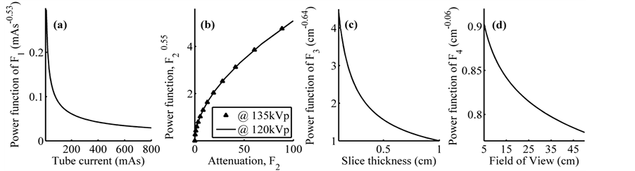
Figure 8. Effect of fractional power functions of quantitative factors: (a) tube current, (b) attenuation, (c) slice thickness and (d) field of view.
[1] -[3] , where the noise is directly proportional to the inverse of the square root of the mAs and the pixel size. The parameter of  does not include the value −0.5 as it could be expected [2] . This confirms the importance of the estimation of model parameters for specific machines of CT, for proper delimitation of optimization strategies and more effective protocols at a radiology department level. Some qualitative factors have not a significant contribution to the noise model, as seen by its parameters:
 ,
,  and
and . The qualitative factors of high resolution mode (HR), “Fine” and “Extra Fine” kernels (RF4 and RF5) contribute also to the increment of the noise, which coefficients are
 ,
,  and
and  respectively, where the mode “HR” influences noise significantly. The remaining modes of reconstruction STD, MAC and 2segs (
 ,
,
 and
and ) and kernels RF1, RF2 and RF3 (
 ,
, 0.61 and
 ) are recommendable for low noise levels.
3.2.3. Validation of Nonlinear Model
The model validation was made by graphical residual analysis. The graphs of dispersion of weighted residuals versus predictor variables are presented from Figure 9 to Figure 10, which do not exhibit any systematic structure, indicating that the model fits well to the data. The graph of weighted residuals considered with lag in Figure 11(a) allows demonstrating the independence of the errors, since there is not a deterministic distribution pattern; the points show a random dispersion. The graph of sequential weighted residuals of Figure 11(b) demonstrates the random behaviour of the same ones; this is due to the fact that the experimental design and the collection of information were randomized.
That is, the measurements were done sequentially without the gradual increase of any factor and the combinations of them were established randomly in the sequence.
In Figure 11(c), it is shown the weighted residuals versus the values of the regression function in order to verify the functional sufficiency of the model. Also they can be used to evaluate the assumption of homoscedasticity of the random errors. The residuals are distributed approximately in equal quantities between the negative and positive values. Systematic patterns are not observed graphically. The probabilistic distribution of weighted residuals is normal, as presented in Figure 11(d), this suggests that the process of estimation of the parameters of the model by NLRR turned out to be optimal.
4. Conclusions
A more inclusive nonlinear model of image noise in CT was obtained. The Least Square Robust Regression constitutes an appropriate method for the estimation of image noise. Further research should be conducted for other image quality descriptors. The product of fractional power functions allows the quantitative analysis of the effect of scanning factors such as tube current, attenuation, slice thickness and FOV. The dependence of image noise from the square root of the inverse of tube current, attenuation and slice thickness was confirmed, but the FOV showed non-significant effect on image noise. Although the functions of the reconstruction algorithms are unknown, the use of binary variables allows to identify their association with the image noise analytically and the estimation of related coefficients for each one.

Figure 9. Graphical analysis of weighted residuals associated with predictors: (a) Tube current F1, (b) attenuation with beam hardening F2, (c) slice thickness F3 and (d) field of view F4.

Figure 10. Graphical analysis of weighted residuals associated with qualitative factors. Reconstruction Modes: (a) Standard X1, (b) High Resolution X2, (c) Motion Compensation X3 and (d) reconstruction of two frames per tube rotation X4. Kernels: (e) Extra smoothing X5, (f) Smooth X6, (g) Standard X7 and (h) Fine X8. Smart Filters: (i) Extra Fine X9, (j) Smooth X10, (k) Middle X11.

Figure 11. Analysis of weighted residuals: (a) with lag = 1, (b) sequential, (c) estimated noise and (d) histogram.
New effective attenuation coefficients were estimated, regarding beam hardening effect on noise, which contributes significantly to noise increase as expected.
The ROI sizes up to 70% of diameter or FOV did not affect the adjusted coefficient of determination, but the parameters of attenuation and FOV showed variations that could lead to physical misinterpretation. A satisfactory ROI size from 30% to 60% was identified. The coefficient of proportionality characterizes how noise-prone can be a CT unit in particular. The type of model proposed provides a tool for identification of alternative protocols with optimisation purposes.