Rural Labor Force Transfer Training Effects Evaluation by Matching Methods: Evidence from Yunnan Province of China ()
1. Introduction
Western regions are the main poverty areas in China, especially the autonomous minority nationality rural areas in the southwestern frontier regions. According to Poverty Monitoring Report of Rural China [1], there were 23.72 million people in poverty in western areas in 2009, which account for 65.9 percent of the country (35.97 million), with only the three of the 31 western provinces: Guizhou, Yunnan and Gansu, exceeding 3 million people in poverty respectively. Incidence of poverty in western regions was 8.3 percent in 2009, an increase of 4.5 percent from the national poverty incidence of 3.8 percent for the same year. In 2009, net income per capita for the western rural poverty population was CNY983, which accounted for 19.1 percent of the total rural population throughout the country.
The autonomous minority nationality rural region had 19.54 million people in poverty in 2009, which accounted for 54.3 percent of all rural people in poverty. The poverty incidence was 16.4 percent in these areas, and 12.6 percent higher than the country poverty incidence. The autonomous minority nationality rural areas were more severely poor than any other areas of the country at the same time period. One of the minority nationality areas is Yunnan province.
Yunnan is the most southwestern province and shares a border of 4060 kilometers with Burma in the west, Laos in the south, and Vietnam in the southeast. It is noted for a very high level of ethnic diversity which has the second highest number of ethnic groups among the provinces in China. Because poverty is widespread in Yunnan and deep-rooted, and the geographical location is special, Yunnan becomes one of the most important poverty alleviation provinces, especially in its costal autonomous minority nationality areas.
A key strategy of poverty alleviation the Chinese government employs is to provide training to the rural largely unskilled working population. In March of 2004, “Suggestions on Accelerating Farmers’ Income by the Party Central Committee and the State Council” was issued and recommended enhancement of the rural labor force through vocational skills training. Thereafter, a series of projects were initiated under the cooperation of the Ministry of Labor and Social Security, the Ministry of Agriculture, the Ministry of Finance, and the Ministry of Education, such as, the Sunshine Project, the Rural Labor Skills Training and Employment Project, and the Rain and Dew Project.
Since the micro survey data are scarce and hard to be obtained, there has been very little evaluation of the rural training programs domestically. Our aim of this study is to evaluate the effects of the rural labor force transfer training program by using Matching methods. The research targets are the Honghe Hani Nationality and Yi Nationality Autonomous Prefecture (Honghe Prefecture) and the Dehong Dai Nationality and Jingpo Nationality Autonomous Prefecture (Dehong Prefecture) of Yunnan province in southwest of China.
This paper is organized as: Section 2 is training participation and income description. A series of matching methods will be introduced in Section 3. Section 4 is empirical results. The last Section is concluding remarks.
2. Training Participation and Income Description
2.1. Data Sources
The data for our study were obtained from the China’s Rural Household Survey (RHS) of Honghe Prefecture and Dehong Prefecture done by local State Statistical Bureau (SSB) offices in Yunnan province. The data appears to be of good quality and bunches of information about rural household income, consumption, production, accumulative and social behaviors. Two-stage sample was selected in each prefecture. The first stage involved the selection of 348 villages from 13 counties of Honghe Prefecture and 5 counties of Dehong Prefecture. In the second stage, it was involved the stochastic sampling of households from the selected villages. There were two main methods have been adopted for collecting data. One is the sampled households fill in a daily diary on expenditures and other relative information. Another one was visiting survey. Sampled households were visited on every month by an interviewer to check the diaries and collect data. Our sample data is a sequence of cross Sections since 2006 and is ongoing. The training information enrolled into this survey only from 2006 to 2008. The survey observations updated every year, tracked the households who appeared in this survey started from 2006 to 2008 continuously, there were 2280 households.
2.2. Training Participants and Their Income
There were 595 (26.10%), 612 (26.84%) and 598 (26.23%) households that had been trained during 2006 to 2008 respectively, the sample average training participation ration is 26.39 percent. In 2007, there were another new 111 households participated and another new 41 households participated in 2008.
Income in this study is net income. In 2008 net income per capita of participants was CNY3841.77 while for non-participators was CNY2690.49. Households participating in training increased the net income almost CNY1000 than those who did not participate in training during these three years. The result shows that household who attended training benefited a lot.
Here the question is that income difference is a result, reasons for income difference could be training, or be other behaviors. It means that statistical description cannot tell whether there has causality between training and income difference. Therefore, it is necessary for us to use Matching methods which are special for cause-and-effect relationship research to estimate training effects in the case of coastal autonomous minority nationality areas of Yunnan province in China.
3. Methodology
The primary question for training programs effects evaluation is: what is the difference between participants’ post-program income and the income that they would have received had they not participated in training [2]. In practice, it is quite difficult to answer this question straightforward. Suppose that there is a target population  has being studied. If we take
  denotes the training status,
  if a farm household participates in training, which is also say a household is treated. Here a household participates in training means any one family member participates in training.
  , denotes a household not participates in training, that is none family member participates. We are interested in income outcome
  and further denote
  as the potential income of participants,
  for non-participator.
  is the treatment effect of the training. The difficulty for effects evaluation is, for a given household, that we observing either
  or
or  at the same time, but not both, this also called missing data problem. In order to overcome this difficulty, we need to structure a counterfactual frame of causality which can be composed by untreated group members and shared with similar observable characteristics of those who are actually treated. Various methods have been employed to solve the above evaluation difficulty, for example, Instrument Variables (IVs) methods [3]; Marginal Treatment Effect (MTE)-based parametric estimations methods and MTE-based semi-parametric estimation methods [4-10]; a series of Matching methods [11-17].
The evaluation method of Matching has been used in many fields since it is easy to understand and easy to apply [3,15,17]. Over the previous literature, there are mainly three popular Matching methods, multivariate Matching based on Mahalanobis Distance (MD) [18-21], Propensity-Score (PS) Matching [11], and Genetic Matching (GenMatch) [15,17,22]. In this research, we will employ these three popular Matching methods to evaluate training effects, and answer the following questions: a) what is the average treatment effect (ATE) for the target population; b) what is the treatment effect of the treated (TT); c) what is the treatment effect of the untreated (TUT); d) which Matching method can reduce bias mostly.
3.1. Parameters of Interests
There are three mean treatment effect parameters:
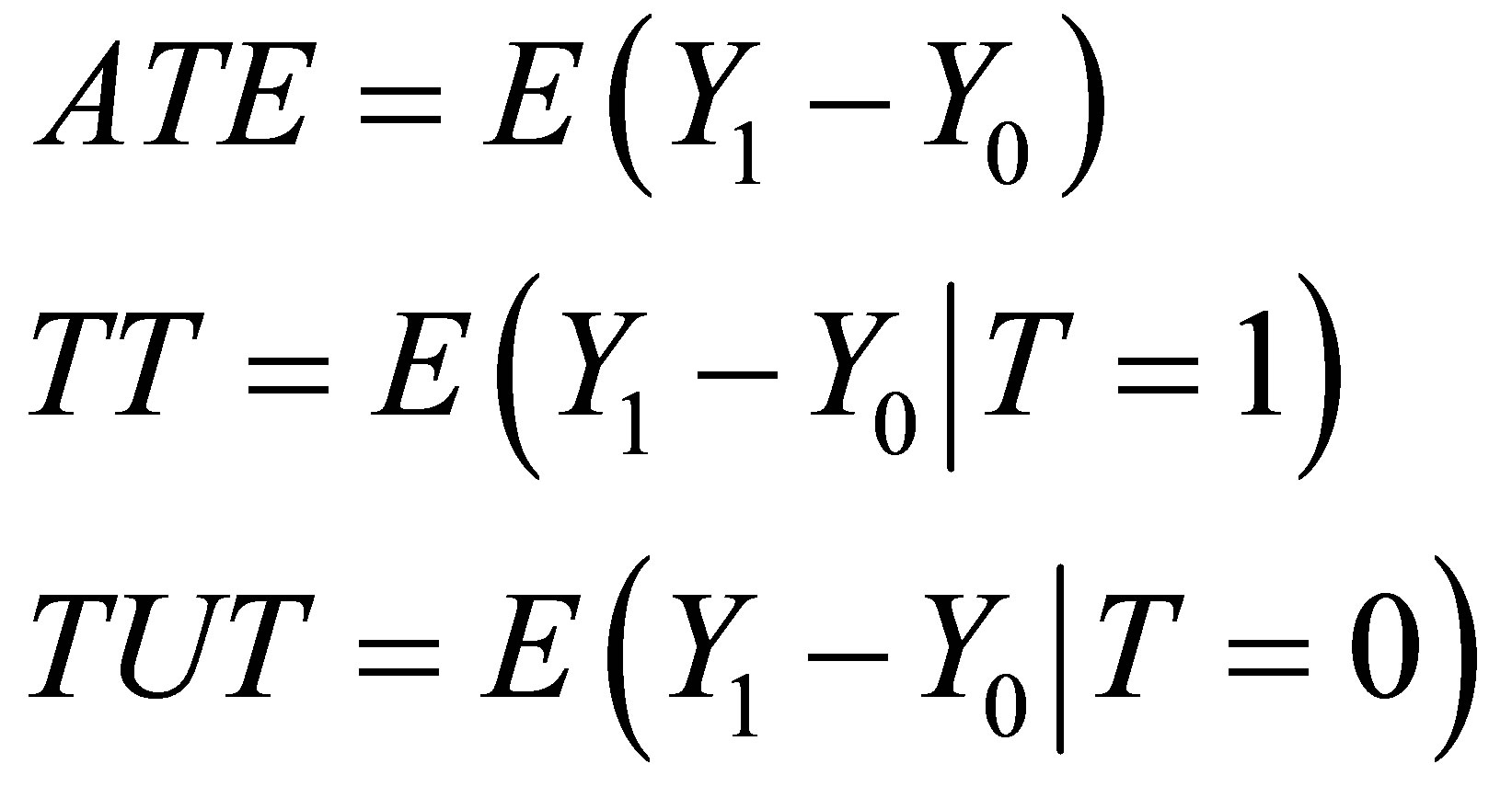
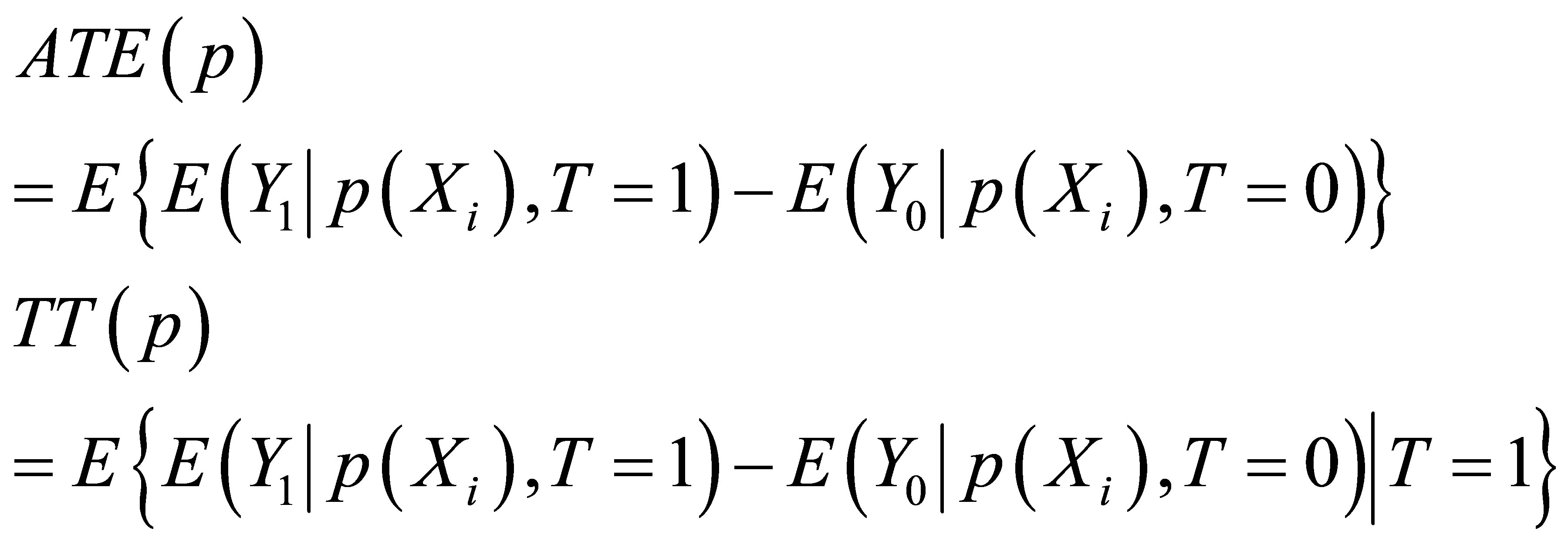
The Average Treatment Effect (ATE) is defined for the whole population. ATE evaluates the average difference between a set of members in  that are randomly selected for treatment and another set of members that are randomly selected for control.
The Treatment effect of the Treated (TT) means to the average difference by treatment status for these people who are treated.
The Treatment effect of the Untreated (TUT) refers to the average difference by treatment status for these who are not treated.
3.2. Matching Based on Mahalanobis Distance Method
As is discussed before, the main difficulty of treatment effect evaluation is the missing data problem and we need to structure a counterfactual frame to overcome this problem. Matching is an excellent tool to structure a counterfactual by filling the missing data for each observation which is similar in terms of their observable characteristics and relies on the Conditional Independence Assumption (CIA) [23] which also has other names, “unconfoundness” or “ignorability” [11], and “exogeneity” [24]. If we let  be a vector of observed covariates, such as education level or whether living in a minority group village in this case, selection to participate in training is independent of potential outcomes, the CIA states:
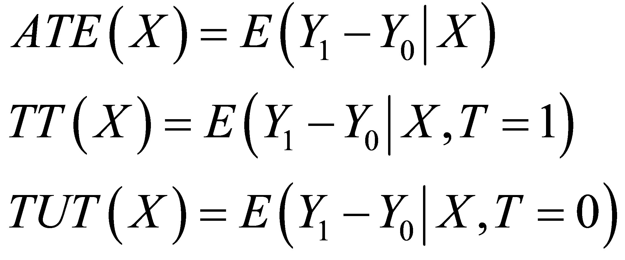
If CIA holds true, the above three parameters of interest ATE, TT and TUT can be expressed as:
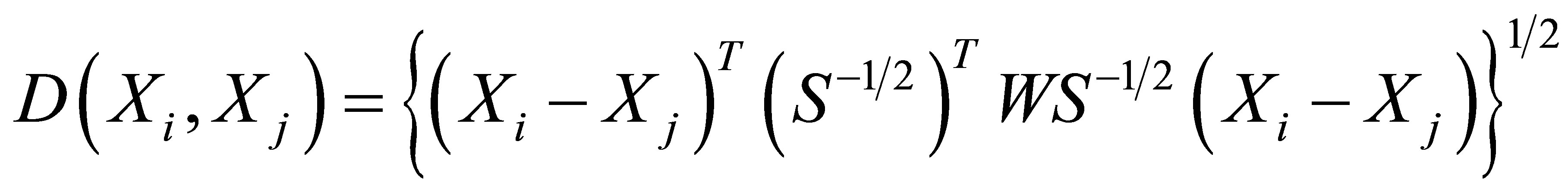
Till now, we can introduce multivariate matching which is based on Mahalanobis Distance to structure a counterfactual for each observation [25]. The Mahalanobis Distance between any two column vectors is:
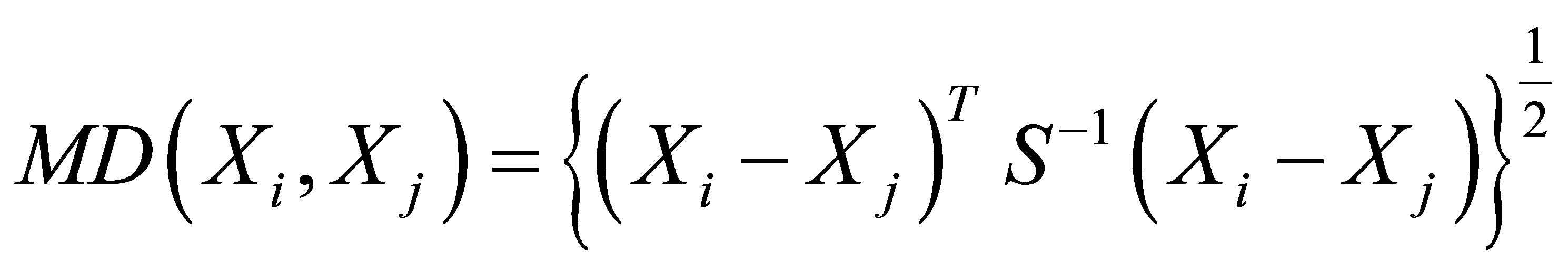
where  is the sample covariance matrix of
  . To estimate TT by matching with replacement, one matches each treated unit with the M closest control units, as defined by this distance measure,
 . Under this method, the estimates will suffer bias when
  consists of more than one continuous variable, which is equivalent to that the multivariate matching results in statistically efficient estimates of the treatment effect only when continuous variables are limited to one [13]. Additional continuous covariates will cause increasingly biased estimates.
A recommended alternative solution for more than one continuous covariate is known as the Propensity Score Matching method.
3.3. Propensity Score Matching Method
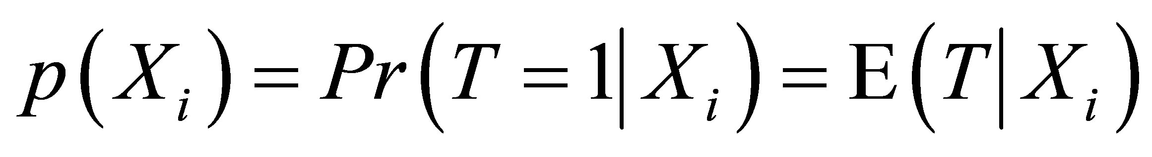
According to Rosenbaum and Rubin [11,26,27], the propensity score which means the probability of receiving treatment conditional on covariates  can reduce the dimensionality of the multivariate matching. Let
  be the probability of a unit
  being treated given
  , which is a household participated in training in this case,
  can be defined as:
Given

and
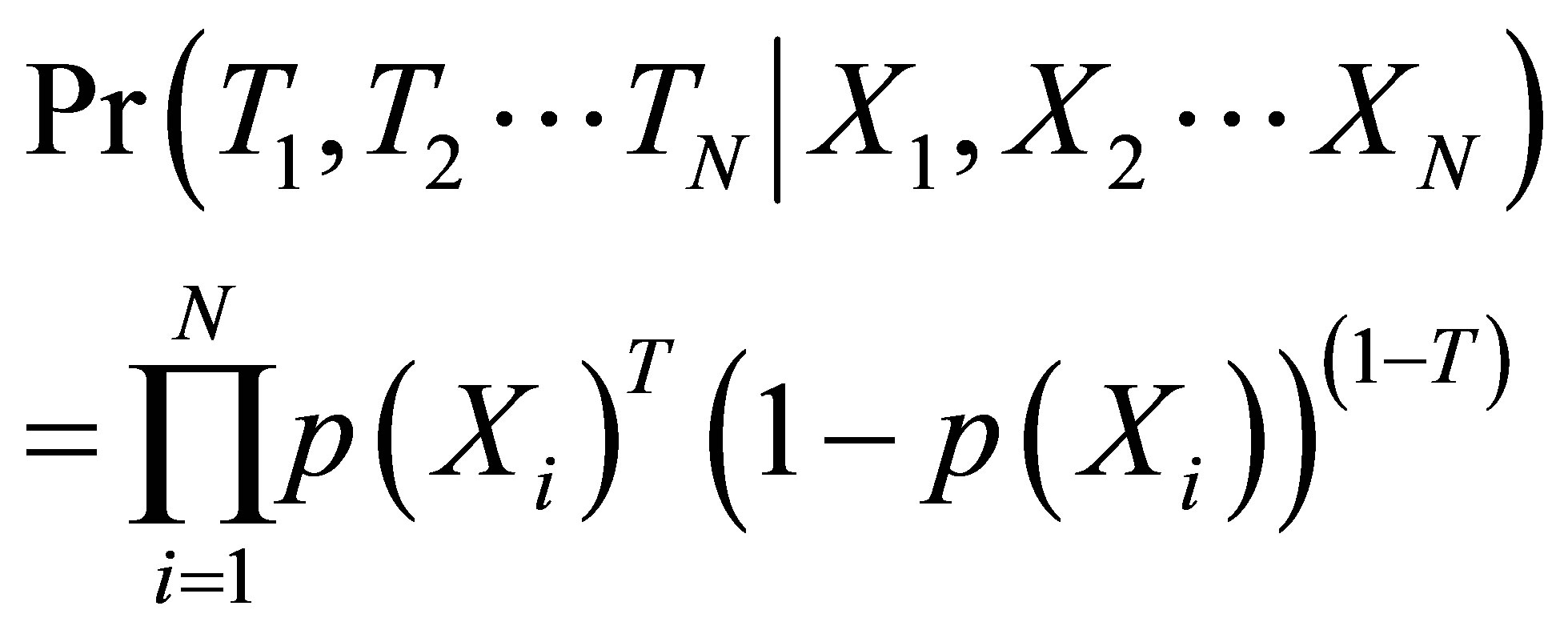
Rosenbaum and Rubin [11] proved that:
The PS Matching differs the matching rule from the MD matching. PS Matching process involves matching as a function of propensity score, which is matching each treated member to the nearest control member on the unidimensional metric of the propensity score vector [28]. If a treatment observation matched with a control observation by matching on a correctly specified propensity score, that will asymptotically balance the observed covariates, and will asymptotically remove the bias conditional on such covariates [11,17]. By covariate balance it means that the treatment and control observations have the same joint distribution of observed covariates [17]. However, in practice, the correct  is unknown, so it must be estimated. Normally,
  can be estimated by using Probit or Logit regression, here we choose Logit regression to estimate
 .
.
The MD Matching and PS Matching can be used alone, or in a way of combination. In this study, we set up different models, Model-1 for the MD Matching, Model-2 for the PS Matching and Model-3 combined the MD Matching with the PS Matching.
3.4. Genetic Matching Method
Genetic Matching (GenMatch) was proposed by Sekhon [17], Diamond and Sekhon [29], with a genetic search algorithm. Since the MD Matching is good at minimizing the distance between treatment and control observations but may fails optimal balance in a given dataset. Therefore, the MD Matching can be extended in a more generalizing method—GenMatch by including an additional weight matrix in the MD matrix:
where  is a
is a  positive definite weight matrix and
  is the Cholesky decomposition of
 , i.e.,
 which is the variance-covariance matrix of
 . All elements of
  are zero except those down the main diagonal and
  parameters must be chosen as the components of the main diagonal. It is easy to see that if each of those
  parameters is equal to one,
  is the same as
  . Sekhon recommend that if one can estimate the propensity score correctly, it should be included as one of the covariates in GenMatch [28]. In this case,
  in
in  might be extended to
  , which is a new matrix consisting of the propensity score
  and
and . It is not hard to understand that GenMatch will be equivalent to PS Matching given a zero weight to covariate
 . Thereby, both the PS Matching and the MD Matching are special cases of GenMatch.
In GenMatch, the genetic search algorithm automates the iterative process by checking and improving balance for each covariate or minimizing imbalance by minimizeing the largest observed covariate discrepancy. Thereby, the imbalance should be small after the optimal matching and it can be measured in a series of methods, such as the nonparametric Kolmogorov-Smirnov(KS)-test statistics and paired t-test and the smallest p-values from KS-tests and t-test, which are need to be large.
In this study, we also set up Model-4 for the GenMatch without propensity score. For each model, we report the covariate balance results to show the effectiveness of each matching method.
4. Empirical Results
4.1. Measures
Based on Mincer income model [30], not only human capital investment has been taken into consideration but also material resources capital investment, farm household characteristics and living village characteristics. We take households who participate in training as the treated group, who not participate in training as the control group. In our research, per capita annual net income  of 2007 has been selected as our outcome variable and been taken logarithm. We did some data processing work before treatment effect evaluation. Since the income variable need to be taken logarithm, we save the households who with positive annual net income. Finally, totally 2053 households who with positive annual net income and participated in training only in 2006 but not in 2007 and 2008 have been selected in our research, in the consideration of the causal inference of training. In addition, there are 570 households in the treated group and 1483 households in the control group. The following Table 1 is variables definition.
4.2. Statistical Analysis
In this research, R software of version 3.0.0 and Matching package are used for the analysis. Firstly, the sample statistical description and the mean differences are calculated with an unpaired Welch Two Sample t-test and are presented in Table 2. For the purpose of finding out the most optimal match for each treated observation, we set up a series models, Model-1 for the MD Matching, Model-2 for the PS Matching, Model-3 for the combination of MD and PS Matching and the last Model-4 for the GenMatch without PS. In each model we match with replacement and one-to-one match because allowing replacement reduces bias.
As is shown in Table 2, totally 27.6 percent modeled sample households participated in training in 2006. Per capita annual net income of treated group is significant higher than which of control group observations and increases from 2006 to 2007. For the highest education level, 56.5 percent of training participants attended junior high school but 47.1 percent for the control group and their difference is 9.4 percent which is significant. We can obtain abundant of information from Table 2, but the most important thing is, the pre-match mean differences are statistical significant between the treated group and
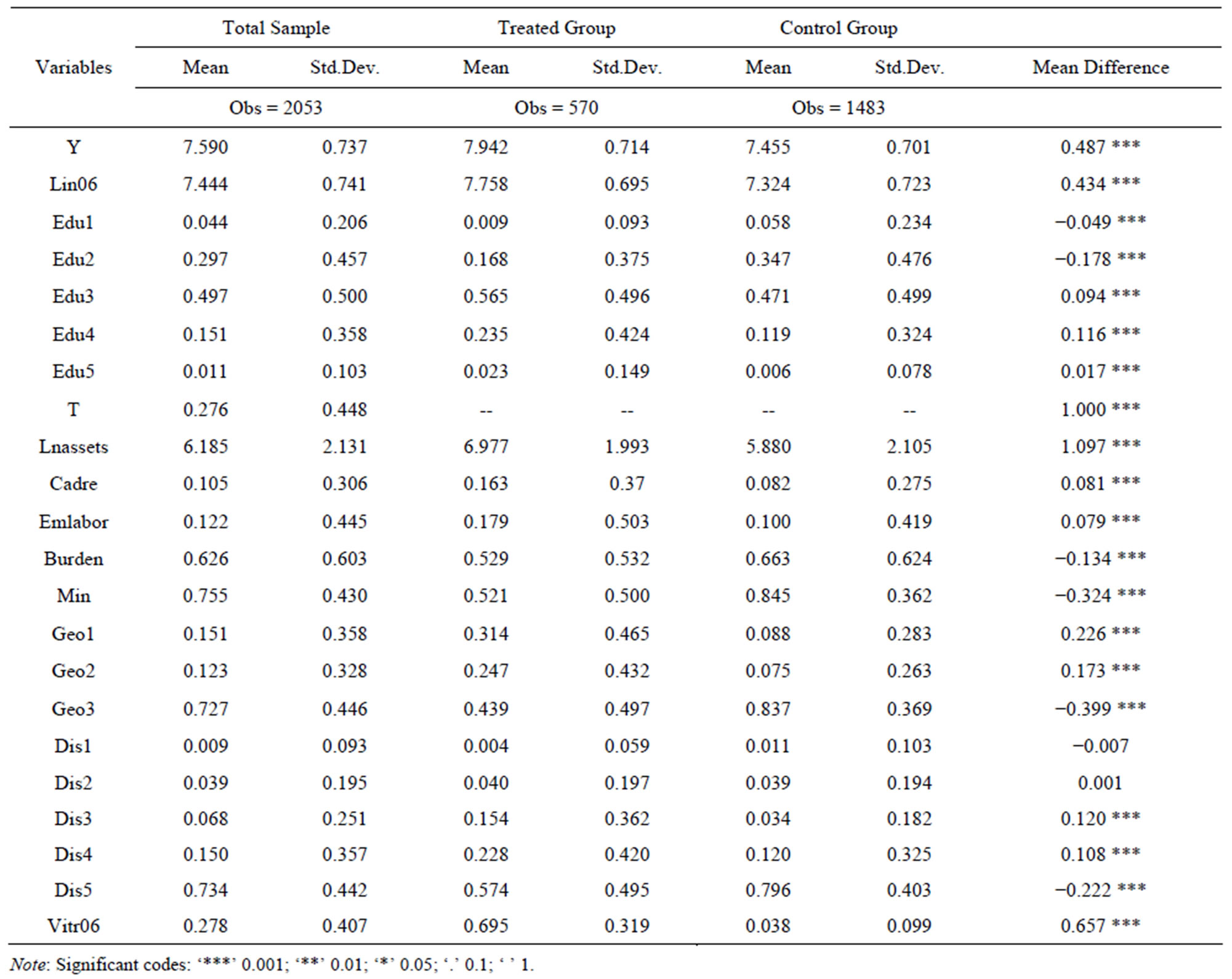
Table 2. Sample statistical description and mean differences.
the control group among most covariates except Dis1 and Dis 2.
4.3. Empirical Results
Before comparing each model, we need to estimate propensity score. As is mentioned before, we choose Logit model to estimate the propensity score and all coefficients estimation presented in Table 3. All the variables in Table 3 are the determinants of the probability of participating in training.
The match balance results of each model which checks whether the results of match have achieved balance on a set of covariance are reported in Tables 4 and 5. For each covariance, kinds of tests and statistics are calculated, i.e. t-test, univariate and multivariate KolmogorovSmirnov (KS) tests and a variety of empirical-QQ plots statistics [28]. But only t-test p-value is reported before and after matching in our study, since for dummy variables, the KS tests results are not provided by the R software and they are the equivalent to the results from t-tests.
The balance results make clear that, each model succeed in reducing covariance differences between the treated and control group at different degrees. Take the Lin06 variable as an example, the balance of it has been
made better by matching. The mean difference is 0.4341 with a p-value of 0.0000 which is statistic significant before matching. After matching, this difference decreases largely in each model and changes to not significant except in Model-1 with the t-test p-value of 0.006. Edu2 variable is balanced after matching in each model, which is what we expected; unfortunately this not happened to every variable. Dis2 variable has been made worse by MD Matching. Before matching, the mean difference is 0.0012 with a p-value of 0.8979, but after matching this mean difference changes to -0.0368 with a p-value of 0.0000 at 0.1 percent significant level. We can check all the balance statistics for every variable followed by the same logic. Then we summarized the comparison result in Table 6.
From Table 6, we can see that, there are totally 20 variables in each model. After matching, there are 14, 3, 13 and 8 variables still imbalanced in each model respectively. In all cases, Model-2 of PS Matching performs with a better balance result than the other three models, since only 3variables still imbalanced after matching, 1variable at the significant level of 5 percent and another 2 variables at the significant level of 1 percent. The results of Model-3 indicates that, combined PS Matching with MD Matching make improvement compared with Model-1, but not so remarkable in this case study. GenMatch make greater progress than the MD Matching, only 2 variables are still significant imbalanced after matching at the level of 0.1 percent versus 8 variables in Model-1.
After matching, the three mean treatment parameters of ATE, TT and TUT and their standard errors are estimated. The results are summarized in Table 7.
As is shown in Table 7, all ATE, TT and TUT estimations are positive and statistical significant in four models. We observe that all three parameters estimation from MD Matching, MD and PS Matching and Genetic Matching are over 20 percent except PS Matching. For TT, the average income difference by treatment status for these farm households who are actually treated is 29.56 percent by MD Matching method, 24.92 percent and 27.35 percent for Model-3 Matching and Model-4 Matching respectively, but only 18.99 percent by the PS Matching method. In each model, the common result of  indicates that the rural labor force transfer training program is well-directed.
From Table 6, we know that the PS Matching performs with an excellent balance result than the other three models. Under this method, TT is 18.99 percent. Compared with this result, the other three matching methods may overestimate the results.
Despite large differences among estimation results by different matching method, from Table 7, we conclude that, firstly, the positive estimation results demonstrate
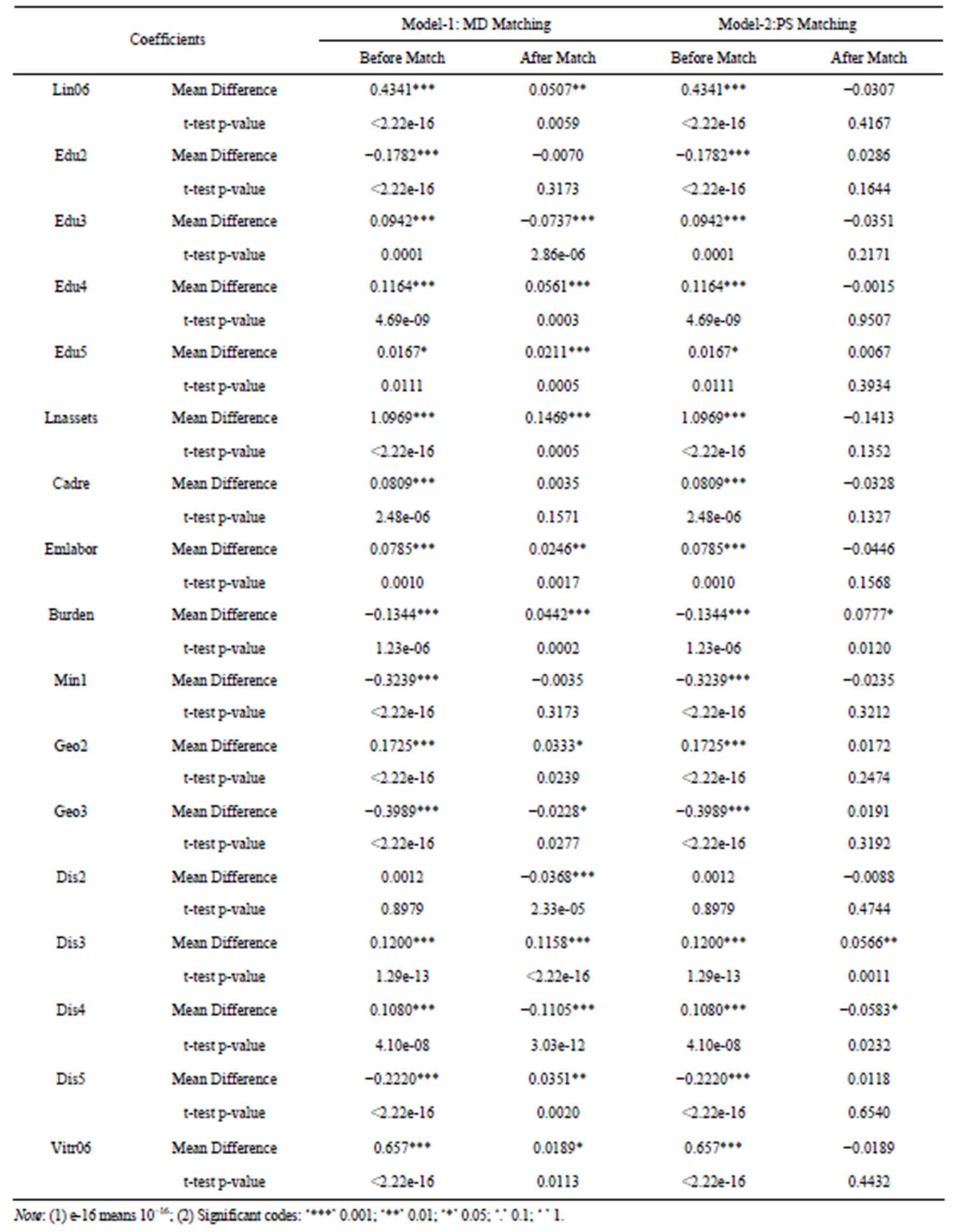
Table 4. Description of the matching balance statistics for Model-1 and Model-2.
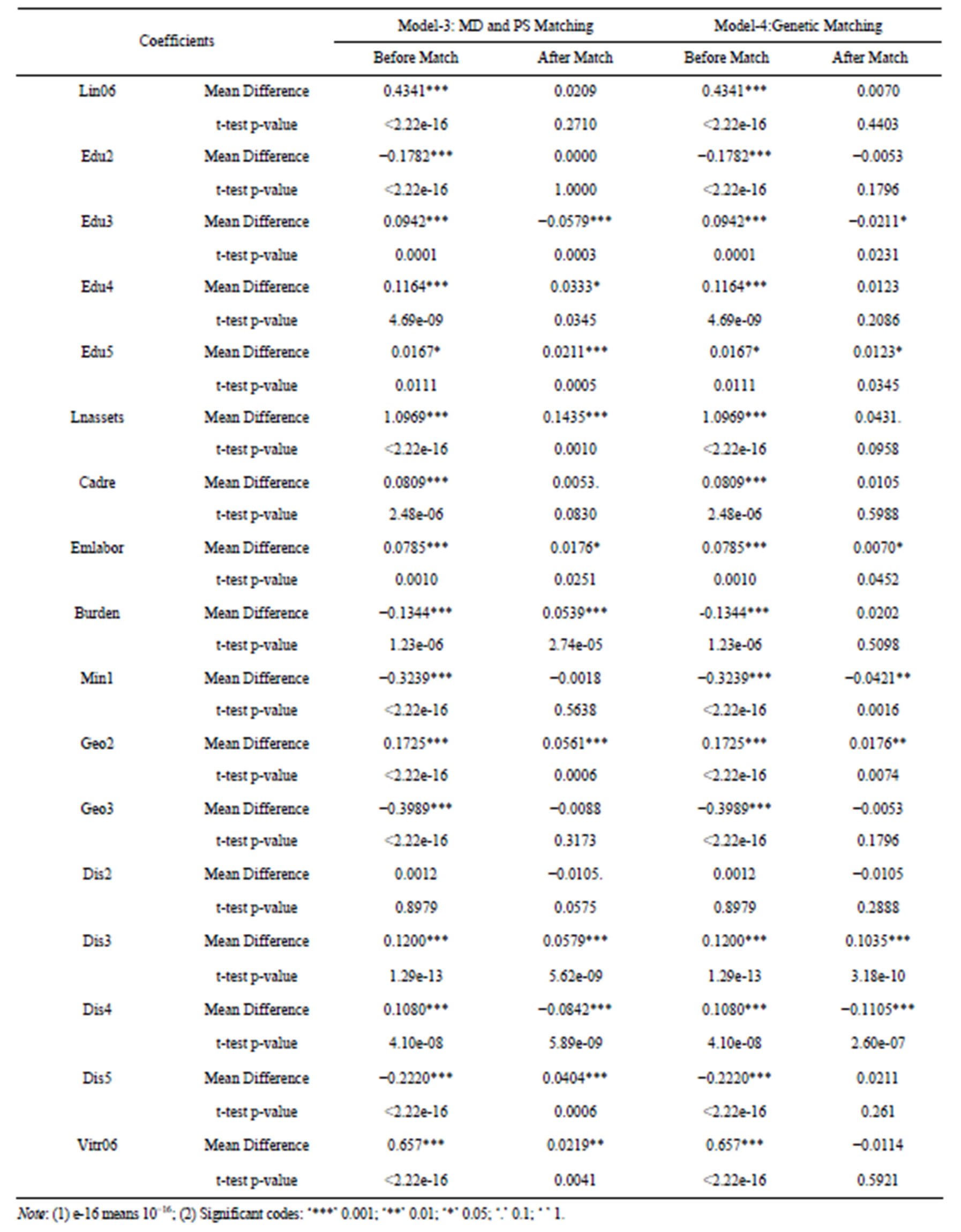
Table 5. Description of the matching balance statistics for Model-3 and Model-4.
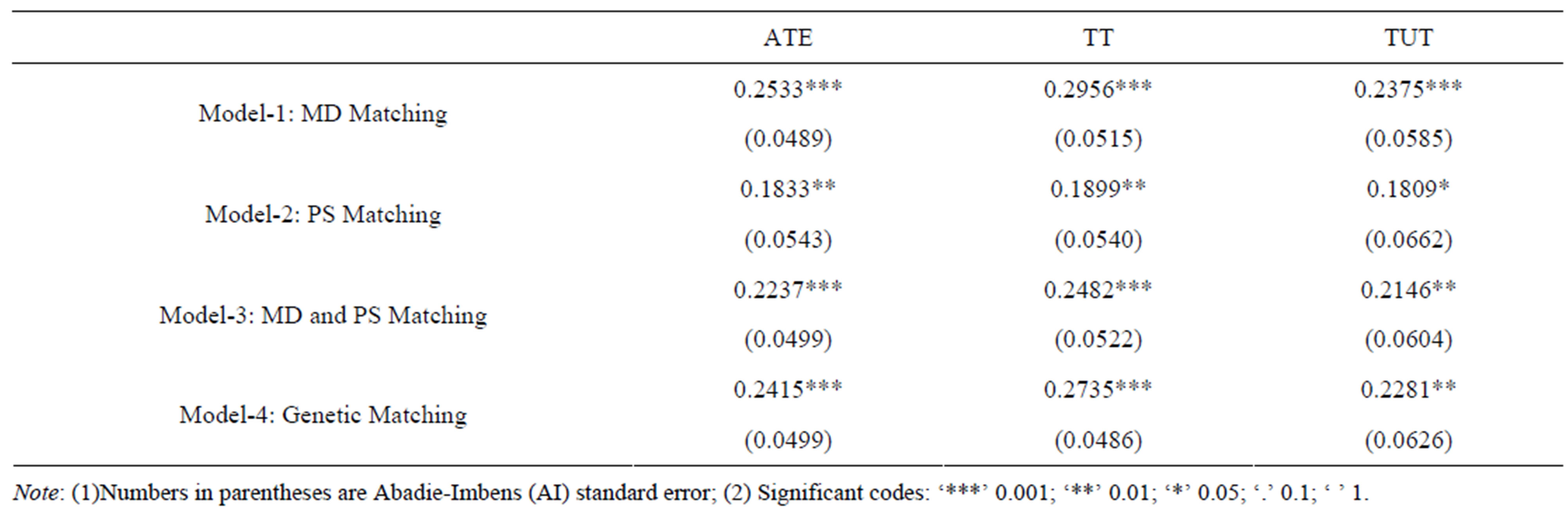
Table 7. ATE, TT and TUT estimation results.
that the rural labor force training program is effective. Secondly, highest TT value illustrates that the rural labor force training program is well-directed.
5. Concluding Remarks
In this study, we use micro data obtained from China’s Rural Household Survey (RHS) of Honghe Prefecture and Dehong Prefecture in Yunnan province, to estimate the Rural Labor Force Training Program effects in the autonomous minority nationality areas in southwestern frontier region of China.
We set up four models with different matching method, and in each model, three treatment effects specified as ATE, TT and TUT are estimated and the results answered the primary question which was proposed at the beginning of section 3 that, what is the difference between participants’ post-program income and the income that they would have received if they haven’t participated in training. The average TT value shows that participants’ income will lose approximately 25.18 percent if they were not participating in training. Under each estimation method, people who participated in training gain the most and gain more than those who are randomly selected if they participated. TUT estimations are less than ATE and TT in each model, and clarify that if nonparticipants are treated, their income will increase. Using our data set, positive ATE, TT and TUT estimations and the largest TT values, demonstrates that the rural labor force training program is effective and well-directed in Honghe Prefecture and Dehong Prefecture.
Our empirical study also provides a good example of using series matching methods. We compared four different matching methods for estimation rural labor force training program policy treatment effects on our sample data and showed the balance checking results with paired t-test p-value. In this empirical study, the Propensity Score Matching reduced imbalance mostly while this conclusion may be inconsistent with other literature. According to Sekhon, Genetic matching with a genetic search algorithm can directly optimize covariate balance even without the propensity score [28,29]. Sekhon estimated TT by Propensity Score Matching and Genetic Matching without propensity score methods using Lalonde experimental data. In his research, Genetic Matching is performed with better balance than Propensity Score Matching. This discrepancy conclusion may be caused by the diverse propensity score model and different constitution of co-variances. Different models give rise to different balance results and it is hard to obtain a correct propensity score model. So we suggest that it is better using a series of matching methods to estimate treatment effects and combining their advantages, rather than only one matching method.
6. Acknowledgements
This work is supported by grants from the National Natural Science foundation of China to the project of “Research of Western Minority Nationality Areas Rural Labor Force Training Program Policy Effects Evaluation and Policy Optimization: Evidence from Yunnan Province of China” (No. 71263055).
NOTES