

Open Access Library Journal
Vol.07 No.02(2020), Article ID:98569,18 pages
10.4236/oalib.1106075
Stability and Adaptive Control with Sychronization of 3-D Dynamical System
Maysoon M. Aziz, Dalya M. Merie
Department of Mathematics, College of Computer Sciences and Mathematics, University of Mosul, Mosul, Iraq

Copyright © 2020 by author(s) and Open Access Library Inc.
This work is licensed under the Creative Commons Attribution International License (CC BY 4.0).
http://creativecommons.org/licenses/by/4.0/



Received: January 14, 2020; Accepted: February 25, 2020; Published: February 28, 2020
ABSTRACT
A three-dimensional system is presented with unknown parameters that employs two nonlinearities terms. The basic characteristics of the system are studied. The stability is measured by Characteristic equation roots, Routh stability criteria, Hurwitz stability criteria and Lapiynov function, all show that the system unstable. Then, Chaoticity is measured by maximum Lapiynov exponent of ( ) and “Kaplan-Yorke” dimension ( ). The system is controlled effectively and synchronized by designed adaptive controllers. Furthermore, the theoretical and graphic results of the system before and after control are compared.
Subject Areas:
Dynamical System
Keywords:
Stabilization, Dissipative System, Adaptive Control, Lapiynov Exponent

1. Introduction
Researches in recent years on chaotic phenomena have increased a lot, because of the increasing frontiers of applications of chaos in engineering and non-engineering systems. “Chaos is a phenomenon which results from the exhibits sensitivity to perturbation in the structural parameters and initial conditions of some classes of dynamical systems” [1]. “Chaotic signals have a random-like nature and broadband spectrum and are non-periodic” [2]. “For a system to be chaotic, the following conditions must be satisfied. Firstly, it must be sensitive to perturbation in its initial conditions which should lead to unpredictability of its future trajectories, secondly, it is not topologically transitive and thirdly, the chaotic orbits are dense in the phase space” [3]. “Among some evolved chaotic attractors in the literature are the Chen’s” [4], “3-D, 4-wing attractor” [5], “Sundarapandian-Pehlivan” [6], “Morphous one parameter attractor” [7], “Rabinovich system” [8]. “When chaotic attractors possess one positive Lapiynov exponent, then the system is chaotic. However, the system which has two or more positive Lapiynov exponents it is a highly chaotic system and becomes hypersensitive to small perturbations in its system dynamics” [9] [10]. “Chaos Control subject has received widespread attention of research because controllability and synchronizability of chaotic attractors are index of utility in different designs such as in secure communications and robotics” [11] [12] [13].
“In the context of stability and stabilization, the principle of Lapiynov stability continued to enjoy large applications; it can effectively stabilize the dissipative systems” [14] [15].
This paper is organized as: Section 2, present a description of 3-d system. Section 3, basic analysis such as stability, dissipativity, Lapiynov dimension ‘‘Kaplan-Yοrke dimension’’. Section 4, we designed adaptive control law of the chaotic system. Section 5, a comparison of the analysis results before and after control. Section 6, we derive results for the adaptive synchronization of identical highly chaotic system. Finally Section 7, summarization of the main results.
2. System Description
A three-dimensional dynamical system [16] consist of three ordinary differential equations with state variables , (i = 1, 2, 3) and four unknown parameters (ρ, α, δ and φ), employs six terms include two quadratic cross-product nonlinear terms. Given by:
(1)
The parameters values are taken as
(2)
3. System Analysis
In this section essential, the system (1) is invested and has the following characteristics.
3.1. Equilibrium Points
The first step to analyze a system is to find its equilibrium points, so we need to solve the nonlinear equations as follows
We get the following equilibrium points:
, ,
3.2. Stability Analysis
3.2.1. Characteristic Equation Roots
“A necessary and sufficient condition for the system to be stable is that the real parts of the characteristic equation have negative real parts”.
When the parameters values are taken as in (2), the Jacobian matrix of system (1) at is:
(3)
By using Horner’s Ruffini method [17] we get:
, ,
Similarly, we find Jacobian matrix at and , then we obtain the eigenvalues, as shown in Table 1.
So the system (1) is unstable.
3.2.2. Routh Stability Criteria
“The system is considered stable by the Routh stability states (all poles in OLHP (Open Loop Half plane)) if and only if all elements of the first column in the Routh array are positive. In addition, number of poles not in the OLHP is equal to the number of sign changes in the first column” [18].
Since, there are two negative elements in the first column. Therefore, the system (1) is unstable.
3.2.3. Hurwitz Stability Criteria
“This criterion is applied using determinants formed from coefficients of the characteristic equation. If the small minors of the square matrix J of the system (1) are all positive then the system (1) is stable, otherwise it’s unstable” [18].
If n = 3 (n denote the degree of the square matrix)
From Equation (3) we find:
Since the values of one minors is less than zero, so the system (1) is unstable.
3.2.4. Lapiynov Function
We can use quadratic function for system (1).
We assume that
(4)
If then the system is stable.
By substituting (1) in Equation (4) we get:
Since therefore the system (1) is unstable.
3.3. Dissipativity
Let , and in the system (1).
Then we get for the vector field
thus the divergence of the vector field V on yields to:
Note that , so the systеm (1) is dissipative for all positive values of , and an exponential rate is:
From above equation, the volume element is contracted by the flow into a volume element at the time t.
3.4. Numerical and Graphical Results
For the numerical solution, we use Runge-Kutta method of order 5th to solve system (1). With initial states
3.4.1. Wave Form of the System (1)
The wave-form for the system (1) is characteristic with non-periodic shape, shown in Figures 1(a)-(c) which is one of the basic characteristic behaviors of chaotic dynamical system.
3.4.2. Phase Portrait of the System (1)
Figures 2(a)-(d) and Figures 3(a)-(c) are shows chaotic attractor for system (1) in , , , space, and 2-D attractor of system (1) in , , plane.
The orbit is dense in each graph which means the system exhibit two-scroll hyper chaotic attractor.

Figure 1. Two-dimension phase planes exhibit chaotic attractor. (a): Time versus ; (b): Time versus ; (c): Time versus .

Figure 2. 3-D Attractor of the system (1).

Figure 3. 2-D Attractor of the system (1).
3.5. Lapiynov Exponent and Lapiynov Dimension
“As a rule the Lapiynov exponents refer to the average exponential rates of divergence or convergence of nearby trajectories in the phase space. The system is chaotic if there is at least one Lapiynov exponent greater than zero”. The values of lapiynov exponents are: ( , and ). Therefore, the Lapiynov dimension ‘‘Kaplan-Yοrke dimension’’ is:
So the system (1) is Highly Chaotic System, as shown in Figure 4.

Figure 4. Lapiynov exponent of system (1).
4. Adaptive Control Strategy
4.1. Theoretical Results
To stabilize highly chaotic system (1), an adaptive control law is designed with unknown parameter α.
As follows:
(5)
when are the feedback controllers.
The adaptive control functions are:
(6)
where the constants , (i = 1, 2,3) are positive , is the parameter estimate of α.
Substituting (6) into (5), we get
(7)
Let the parameter estimation error
(8)
Using (8), the dynamics (7) can be written compactly as
(9)
The Lapiynov approach is used for derivation of update law for adjusting the parameter estimate .
Consider the lapiynov function
(10)
Notice V is positive-definite on .
Also
(11)
Differentiating V with substituting (9) and (11), we get:
(12)
In Equation (12), we update estimated parameter by:
(13)
where the constant is a positive.
Now, we substitute (13) into (12), we obtain
(14)
Notice is negative definite on .
Thus, by lapiynov stability, Routh-array criteria, Eigenvalues and Hurwitz stability criteria we get the below result.
Proposition 1. The chaotic system (5) with unknown parameter is stabilized for every initial value by adaptive control (6), where the estimated parameter is obtained by (13) and are greater than zero.
4.2. Numerical Results
To simulate the controlled highly chaotic system (7) we take the initial values and .
Figure 5 shows Controlled trajectories of system (1).
5. System Comparison Tables before & after Control
See Tables 1-6.

Figure 5. Controlled state trajectories of system (1).
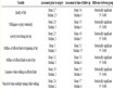
Table 1. Eigenvalues of the system (1) before and after control.
Table 2. Hurwitz criteria of the system (1) before and after control.
Table 3. Routh array criteria of the system (1) before and after control.
Table 4. Lapiynov function of system (1) before and after control.
Table 5. Lapiynov exponent of system (1) before and after control.
Table 6. Of phase portrait of the system (1) before and after control.
6. Adaptive Synchronization Technique
6.1. Theoretical Results
We apply adaptive synchronization technique of highly chaotic system with unknown parameter α.
The drive system is
 (15)
(15)
where , (i = 1, 2, 3) are state variables.
As the response system, the controlled highly chaotic dynamics given by
 (16)
(16)
where  are nonlinear controllers to be designed, and the state variables are
 , (i = 1, 2, 3).
The synchronization error is defined by
 (17)
(17)
then the error dynamics is obtained as
 (18)
(18)
The adaptive control functіοns  define as
 (19)
(19)
where the constants  greater than zero, and
  is the estimated value of the parameter α.
Substitute (19) into (18), to obtain the error dynamics as
 (20)
(20)
Now, the parameter estimation error is
 (21)
(21)
By substituting (21) into (20), the error dynamics simplifies to
 (22)
(22)
From Lapiynov approach we derive the updated law to adjust the estimation of the parameter.
The quadratic lapiynov function is
 (23)
(23)
which be a positive definite on .
.
Note that
 (24)
(24)
Differentiating V and substituting (22) & (24) in it, we get:
 (25)
(25)
update the estimated parameter in Equation (25) by the following
 (26)
(26)
where the constant  is greater than zero.
From (25) and (26), we obtain:
 (27)
(27)
We note that (27) is negative definite on .
.
Hence, by Lapiynov stability [14], “it is immediate that the parameter error and synchronization error decay exponentially to zero with time for all initial values”.
Thus, we proved the results below.
Proposition 2. The drive and response identical chaotic systems (15) and (16) with unknown parameter α are synchronized for all initial values by adaptive control law (19), where the estimated parameter given by (26) and  are constants greater than zero.
6.2. Numerical Results
To get the results numerically, we used the 4th-order Runge-Kutta method to solve systems (15) & (16), and solve system (18) with adaptive control law (19).
We take  and
and  as initial states of the drive system (15) and the response system (16) respectively. Also take α = 296.5 and
  for i = 1, 2, 3, 4.
Figure 6 shows adaptive synchronization of the highly chaotic system.
Figure 7 shows the convergent for system (18) with controller (19).
7. Conclusion
A three-dimensional dynamical system is dealt in this paper, it has quadratic cross-product nonlinear terms. The basic characteristics are analyzed by equilibrium points, stability analysis (such as characteristic equation roots, Routh criterion, Hurwitz criterion and Lapiynov function) all methods of stability shows that the system is unstable. Then, dissipativity analysis indicates system (1) is dissipative for positive values of the parameter . Lapiynov exponent, lapiynov dimension and wave-form analysis present the hyper chaos behavior when the

Figure 6. The synchronization trajectories for system (15) and (16).

Figure 7. The convergent for system (18) with adaptive control (19).
parameters taken as , and the maximum values of lyapenov exponents are:
 ,
,  and
and , lapiynov dimension “Kaplan-Yοrkе dimension” of the system is
 , which means that the system is highly chaotic system. Moreover, to stabilize the highly chaotic system, we produced an adaptive control strategy. Finally, we proposed adaptive synchronization scheme for identical highly chaotic system with upadate law for the estimiation of system parameter. Synchronization schemes are established by Lapiynov stability. Furthermore, we compared theoretical and graphical results of the system before and after control.
Conflicts of Interest
The authors declare no conflicts of interest regarding the publication of this paper.
Cite this paper
Aziz, M.M. and Merie, D.M. (2020) Stability and Adaptive Control with Sychronization of 3-D Dynamical System. Open Access Library Journal, 7: e6075. https://doi.org/10.4236/oalib.1106075
References
- 1. Cuomo, K.M., Oppenheim, A.V. and Strogatz, H.S. (1993) Synchronization of Lorenz-Based Chaotic Circuits and Application to Secure Communication. IEEE Transaction on Circuits and Systems-II: Analogue and Digital Processing, 40, 626-633.
https://doi.org/10.1109/82.246163 - 2. Jovic, B. (2011) Synchronization Techniques for Chaotic Communication Systems. Springer-Verlag, Berlin, Heidelberg.
https://doi.org/10.1007/978-3-642-21849-1 - 3. Volos, C.K., Kyprianidis, I.M. and Stouboulos, I.N. (2012) A Chaotic Path Planning Generator for Autonomous Mobile Robots. Robotics and Autonomous Systems, 60, 651-656. https://doi.org/10.1016/j.robot.2012.01.001
- 4. Chen, G. and Ueta, T. (1999) Yet Another Chaotic Attractor. International Journal of Bifurcation and Chaos, 9, 1465-1466.
https://doi.org/10.1142/S0218127499001024 - 5. Yu, F. and Wang, C. (2013) Generation of a New Three-Dimensional Autonomous Chaotic Attractor and Its Four Wing Type. Engineering Technology and Applied Science Research, 3, 352-358.
- 6. Sundarapandian, V. and Pehlivan, I. (2012) Analysis, Control, Synchronization and Circuit Design of a Novel Chaotic System. Mathematical and Computer Modelling, 55, 1904-1915. https://doi.org/10.1016/j.mcm.2011.11.048
- 7. Wang, X., Chen, J., Lu, J.-A. and Chen, G. (2011) A Simple Yet Complex One-Parameter Family of Generalized Lorenz-Like Systems. https://doi.org/10.1142/S0218127412501167>www.arXiv:1101.4262v3
https://doi.org/10.1142/S0218127412501167 - 8. Pikovsky, A.S., Rabinovich, M.I. and Traktengerts, V.Y. (1978) Onset of Stochasticity in Decay Confinement of Parametric Instability. Soviet Physics: JETP, 47, 715-719.
- 9. Aziz, M.M. and AL-Azzawi, S.F. (2017) Hybrid Chaos Synchronization between Two Different Hyperchaotic Systems via Two Approaches. Optik, 138, 328-340.
https://doi.org/10.1016/j.ijleo.2017.03.053 - 10. AL-Azzawi, S.F. and Aziz, M.M. (2018) Chaos Synchronization of Nonlinear Dynamical Systems via a Novel Analytical Approach. Alexandria Engineering Journal, 57, 3493-3500. https://doi.org/10.1016/j.aej.2017.11.017
- 11. Aziz, M.M. and AL-Azzawi, S.F. (2016) Control and Synchronization with Known and Unknown Parameters. Applied Mathematics, 7, 292-303.
https://doi.org/10.4236/am.2016.73026 - 12. AL-Azzawi, S.F. and Aziz, M.M. (2019) Strategies of Linear Feedback Control and Its Classification. Telkomnika (Telecommunication, Computing, Electronics and Control), 17, 1931-1940. https://doi.org/10.12928/telkomnika.v17i4.10989
- 13. Nakamura, Y. and Sekiguchi, A. (2001) The Chaotic Mobile Robot. IEEE Transactions on Robotics and Automation, 17, 898-904. https://doi.org/10.1109/70.976022
- 14. Hahn, W. (1967) The Stability of Motion. Springer, New York.
https://doi.org/10.1007/978-3-642-50085-5 - 15. Sundarapandian, V. and Sivaperumal, S. (2011) Global Chaos Synchronization of Hyperchaotic Chen Systems by Sliding Mode Control. International Journal of Engineering Science and Technology, 3, 4265-4271.
- 16. Srisuchinwong, B. and Munmuangsaen, B. (2010) A Highly Chaotic Attractor for a Dual-Channel Single Attractor, Private Communication System. Proceedings of the Third Chaotic Modeling and Simulation International Conference, Chania, Crete, Greece, June 2010, 177-184. https://doi.org/10.1142/9789814350341_0046
- 17. Cajori, F. (1911) Horner’s Method of Approximation Anticipated by Ruffini. Bulletin of the American Mathematical Society, 17, 409-414.
- 18. Joseph, J. and Allen, I. (1990) Feedback and Control Systems. McGraw-Hill, New York.