Engineering
Vol.5 No.5A(2013), Article ID:31864,13 pages DOI:10.4236/eng.2013.55A009
Higher-Order WHEP Solutions of Quadratic Nonlinear Stochastic Oscillatory Equation
1Department of Engineering Mathematics & Physics, Engineering Faculty, Cairo University, Giza, Egypt
2Department of Applied Mathematics, College of Science, Northern Borders University, Arar, KSA
3College of Home Economics, Northern Borders University, Arar, KSA
Email: zbeltagy@eng.cu.edu.eg, xxwhitelinnetxx@hotmail.com
Copyright © 2013 Mohamed A. El-Beltagy, Amnah S. Al-Johani. This is an open access article distributed under the Creative Commons Attribution License, which permits unrestricted use, distribution, and reproduction in any medium, provided the original work is properly cited.
Received February 25, 2013; revised March 28, 2013; accepted April 7, 2013
Keywords: Oscillatory Equation; Nonlinear Differential Equations; Stochastic Differential Equation; Wiener-Hermite Expansion; Perturbation Technique
ABSTRACT
This paper introduces higher-order solutions of the quadratic nonlinear stochastic oscillatory equation. Solutions with different orders and different number of corrections are obtained with the WHEP technique which uses the WienerHermite expansion and perturbation technique. The equivalent deterministic equations are derived for each order and correction. The solution ensemble average and variance are estimated and compared for different orders, different number of corrections and different strengths of the nonlinearity. The solutions are simulated using symbolic computation software such as Mathematica. The comparisons between different orders and different number of corrections show the importance of higher-order and higher corrected WHEP solutions for the nonlinear stochastic differential equations.
1. Introduction
Analysis of the response of linear and nonlinear systems subjected to random excitations is of considerable interest to the fields of mechanical and structural engineering [1]. Stochastic differential equations based on the white noise process provide a powerful tool for dynamically modeling complex and uncertain aspects. In many practical situations, it is appropriate to assume that the nonlinear term affecting the phenomena under study is small enough; then its intensity is controlled by means of a frank small parameter, say ![]() [2].
[2].
According to [3], the solution of stochastic partial differential equations (SPDEs) using Wiener-Hermite expansion (WHE) has the advantage of converting the problem to a system of deterministic equations that can be solved efficiently using the standard deterministic numerical methods. The main statistics, such as the mean, covariance, and higher order statistical moments, can be calculated by simple formulae involving only the deterministic Wiener-Hermite coefficients. In WHE approach, there is no randomness directly involved in the computations. One does not have to rely on pseudo random number generators, and there is no need to solve the stochastic PDEs repeatedly for many realizations. Instead, the deterministic system is solved only once.
The application of the WHE [4-10] aims at finding a truncated series solution to the solution process of a stochastic differential equation. The truncated series composes of two major parts; the first is the Gaussian part which consists of the first two terms, while the rest of the series constitute the non-Gaussian part. In non-linear cases, there exists always difficulties of solving the resultant set of deterministic integro-differential equations got from the applications of a set of comprehensive averages on the stochastic integro-differential equation obtained after the direct application of WHE. Many authors introduced different methods to face these obstacles. Among them, the WHEP technique [4] was introduced using the perturbation technique to solve perturbed nonlinear problems.
The WHE was originally started and developed by Norbert Wiener in 1938 and 1958 [11]. Wiener constructed an orthonormal random bases for expanding homogeneous chaos depending on white noise, and used it to study problems in statistical mechanics. Cameron and Martin [12] developed a more explicit and intuitive formulation for Wiener-Hermite expansion (now it is known as Wiener Chaos Expansion, WCE). Their development is based on an explicit discretization of the white noise process through its Fourier expansion, which was missed in Wiener’s original formalism. This approach is much easier to understand and more convenient to use, and hence replaced Wiener’s original formulation. Since Cameron and Martin’s work, WHE has become a useful tool in stochastic analysis involving white noise (Brownian motion) [3]. Also, another formulation was suggested and applied by Meecham and his co-workers [13, 14]. They have developed a theory of turbulence involving a truncated WHE of the velocity field. The randomness is taken up by a white-noise function associated, in the original version of the theory, with the initial state of the flow. The mechanical problem then reduces to a set of coupled integro-differential equations for deterministic kernels. In [1], the WHE (Imamura formulation, [13]) was used to compute the nonstationary random vibration of a Duffing oscillator which has cubic nonlinearity under white-noise excitation. Solutions up to second order are obtained by solving the equivalent deterministic system by an iterative scheme. M. El-Tawil and his coworkers [4-10] used the WHE together with the perturbation theory (WHEP technique) to solve a perturbed nonlinear stochastic diffusion equation.
As in [15], the analysis of nonlinear random vibration has been studied using several methods, such as, equivalent linearization method [16], stochastic averaging method [17], the WHE approach with nonstationary excitations [1], the WHE method combining with the small perturbation technique [18], eigenfunction expansions [19], and the method of detailed balance [20]. All the above methods are applied and used for nonlinear random oscillations of real systems subjected to random nonstationary (or stationary) excitations.
As in [5,6], quadrate oscillation arises through many applied models in applied sciences and engineering when studying oscillatory systems [21]. These systems can be exposed to a lot of uncertainties through the external forces, the damping coefficient, the frequency and/or the initial or boundary conditions. These input uncertainties cause the output solution process to be also uncertain. For most of the cases, getting the probability density function (p.d.f.) of the solution process may be impossible. So, developing approximate techniques (through which approximate statistical moments can be obtained) is an important and necessary work. There are many techniques which can be used to obtain statistical moments of such problems. The main goal of this paper is to compare some of these methods when applied to a quadrate nonlinearity problem.
In [22], the WHEP technique is generalized to nth nonlinearity, general order of WHE and general number of corrections. Also, the extension to handle white noise in more than one variable and general nonlinearities are outlined. The generalized algorithm is implemented and linked to MathML [23] script language to print out the resulting equivalent deterministic system.
In the current work the generalized WHEP technique developed in [22] is used to derive higher-order with higher corrections system of equations for the quadratic nonlinear stochastic oscillatory equation and then solve them. Up to fourth order equations are derived with different number of corrections. The mean and variance of the response will be simulated up to third order using Mathematica.
This paper is organized as follows. The formulation of the quadratic nonlinear stochastic oscillatory equation is outlined in Section 2. The WHEP technique is reviewed in Section 3. The equivalent deterministic system is derived in Section 4. In Section 5, the mean and variance of the solution is simulated with different order, different number of corrections and different values of the nonlinearity strengths.
2. Problem Formulation
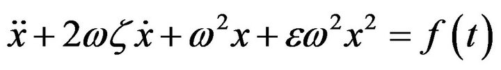
In this paper, the nonlinear oscillatory equation:
 (1)
(1)
is considered under stochastic excitation and with the proper set of initial conditions  which is assumed to be deterministic. The operator L is a general linear operator and in the case of the oscillatory equation it will be:

where ![]() is the undamped angular frequency of the oscillator and
is the undamped angular frequency of the oscillator and ![]() is the damping ratio. The nonlinearity is introduced as losses of degree
is the damping ratio. The nonlinearity is introduced as losses of degree  strengthened by a deterministic small parameter
 . The uncertainty is introduced through white noise scaled by a deterministic envelope function
 . The white noise is considered here as a function of time but it can be generalized in time and space as it was declared in [22]. The function
  is a deterministic forcing function. Theorem (1) will be used in the derivation of the WHEP technique.
Theorem (1): The solution of Equation (1), if exists, is a power series in![]() , i.e.
, i.e.
 (2)
(2)
The theorem can be proved using the mathematical induction with the Pickard iterative technique [22]. As a direct result of this theorem, it is expected that the average, the variance as well as the covariance are also power series of![]() .
.
The WHEP technique will be used in this work to determine the equivalent deterministic set of equations. The deterministic equations are then solved to obtain the solution kernels and hence the mean and variance of the response.
3. WHEP Technique
As a consequence of the completeness of the WienerHermite set [13], any arbitrary stochastic process can be expanded in terms of the Weiner-Hermite polynomial set and this expansion converges to the original stochastic process with probability one.
The solution function  can be expanded in terms of Wiener-Hermite functionals as [4]:

Or after eliminating the parameters, for the sake of brevity, we get:
 (3)
(3)
where  and
and  is a k-dimensional integral over the variables
 . The first term in the expansion (3) is the non-random part or ensemble mean of the function. The first two terms represent the normally distributed (Gaussian) part of the solution. Higher terms in the expansion depart more and more from the Gaussian form. The Gaussian approximation is usually a bad approximation for nonlinear problems, especially when high order statistics are concerned [3].
The components  are called the (deterministic) kernels of the WHE for
 . The variable w is a random output of a triple probability space
 , where
  is a sample space,
  is a
is a ![]() - algebra associated with
- algebra associated with  and P is a probability measure. For simplicity,
 ![]() will be dropped later on.
will be dropped later on.
The functional  is the
  order Wiener-Hermite time-independent functional. The Wiener-H functionals form a complete set with
  and
and : the white noise. By construction, the Wiener-Hermite functions are symmetric in their arguments and are statistically orthonormal, i.e.

The average of almost all Wiener-Hermite functionals vanishes, particularly,

The expectation and variance of the solution will be:
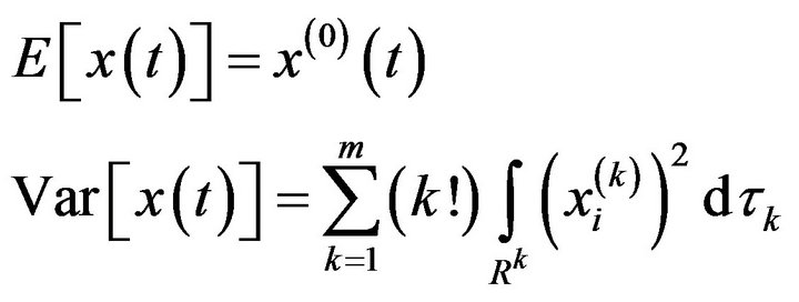 (4)
(4)
The WHE method can be elementary used in solving stochastic differential equations by expanding the solution as well as the stochastic input processes via the WHE. The resultant equation is more complex than the original one due to being a stochastic integro-differential equation [4]. Taking a set of ensemble averages together with using the statistical properties of the WHE functionals, a set of deterministic integro-differential equations are obtained in the deterministic kernels  To obtain approximate solutions of these deterministic kernels, one can use perturbation theory in the case of having a perturbed system depending on a small parameter
![]() . Expanding the kernels as a power series of
. Expanding the kernels as a power series of![]() , another set of simpler iterative equations in the kernel series components are obtained. This is the main idea of the WHEP algorithm.
, another set of simpler iterative equations in the kernel series components are obtained. This is the main idea of the WHEP algorithm.
The WHEP technique for general nonlinear exponent![]() , general order
, general order ![]() and general number of corrections
and general number of corrections  follow the steps [22]:
1. Truncate the expansion (3) to contain only
 kernels
 , i.e.
 and then 2. Substitute into the stochastic partial differential Equation (1);
3. Use the multinomial theorem to expand the nonlinear term  in (1);
4. Multiply by  and then apply the ensemble average. This will lead to
  equations in the kernels
 ;
;
5. For each kernel , apply the perturbation technique up to
  corrections, i.e.
 ;
;
6. Equating the coefficients of  in both sides to get
  equations for each kernel
  .
.
This will lead to the following  equations [22]:
 (5)
(5)
 (6)
(6)
where
 (7)
(7)
And the expectations  are computed as:
 (8)
(8)
It was explained in [22] how to get  in terms of the Dirac delta functions and then use them to reduce the integrals appear in
 . The summation
  means that all variations
  that satisfy the equality
  are selected. This can be done be a searching technique. For these variations, the factors
  will be multiplied by each other to get
  i.e.
i.e. . The term
  is the Kronecker delta function that equals one when
  and zero otherwise. Similarly, the term
  is the Kronecker delta function that equals one when
  and zero otherwise. The counter
 , in the summation in the right hand side of (6), runs over all the
  combinations of the positive integers
  such that
 .
.
Equations (5) and (6) can always be solved using the proper sequence. The first  Equations (5) are solved independently to get
  then they are used to compute the other components in (6). For
 , the component
  is obtained by solving
 with the original initial conditions which are assumed deterministic. For
 , the component
 is obtained by solving
  with zero initial conditions. The other components
  will be zeros due to zero right hand side and zero initial conditions. Equations (6) specify the solution sequence to be followed. The component
  is evaluated in terms of the previously computed components
 . This means that the 1st corrections for all kernels,
  are solved firstly then solving the 2nd corrections for all kernels,
  ,
,
 up to the
  corrections for all kernels
 .
.
These results are consistent with the known results obtained using WHE. In WHE, higher order kernels are driven by lower order kernels, and at the bottom, the Gaussian kernels are driven by the random forcing directly. So, the lower order kernels are usually dominant in magnitude [3].
The statistical properties of the solution will now be calculated as:
 (9)
(9)
If , then it will be convergent if [22]:
for . This means that
  should obey an upper bound condition after which divergence is obtained.
The formulation given in Equations (5) and (6) are quite general and could be used for analysis of the response of an any linear operator ![]() with
with  degree nonlinearity and subjected to an arbitrary, stationary, or nonstationary Gaussian or non-Gaussian random excitation.
Consider the quadratic  nonlinear oscillatory equation with excitation function:
 (10)
(10)
With the initial conditions

In case of zero initial conditions, the exact solution can be obtained using different methods such as the theory of linear differential equations or the Laplace transform, and it will be the convolution:
 (11)
(11)
where 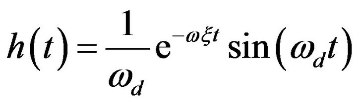 with
with which is the angular frequency of the underdamped
  harmonic oscillator.
For , the solution will results in:

The solution (11) of the model Equation (10) can be used as a model solution that is used in all kernels after considering the proper right hand side for the kernel equation.
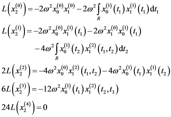
4. The Equivalent Deterministic System
Applying the above mentioned WHEP algorithm to get the following systems of equations of the quadratic (n = 2) nonlinear oscillatory equation and first order (m = 1) Gaussian approximation and different number of corrections . The initial conditions are assumed deterministic and hence only the zero-order and zerocorrection kernel equation
  will has the initial conditions
 . Other kernels equations will have zero initial conditions.
 :
:

 : The above equations in addition to:

 : The above equations in addition to:

 : The above equations in addition to:

 : The above equations in addition to:

In case of zero initial conditions and zero deterministic excitation [i.e. ], we shall have:
Which means the all of  and
and  are become zeros.
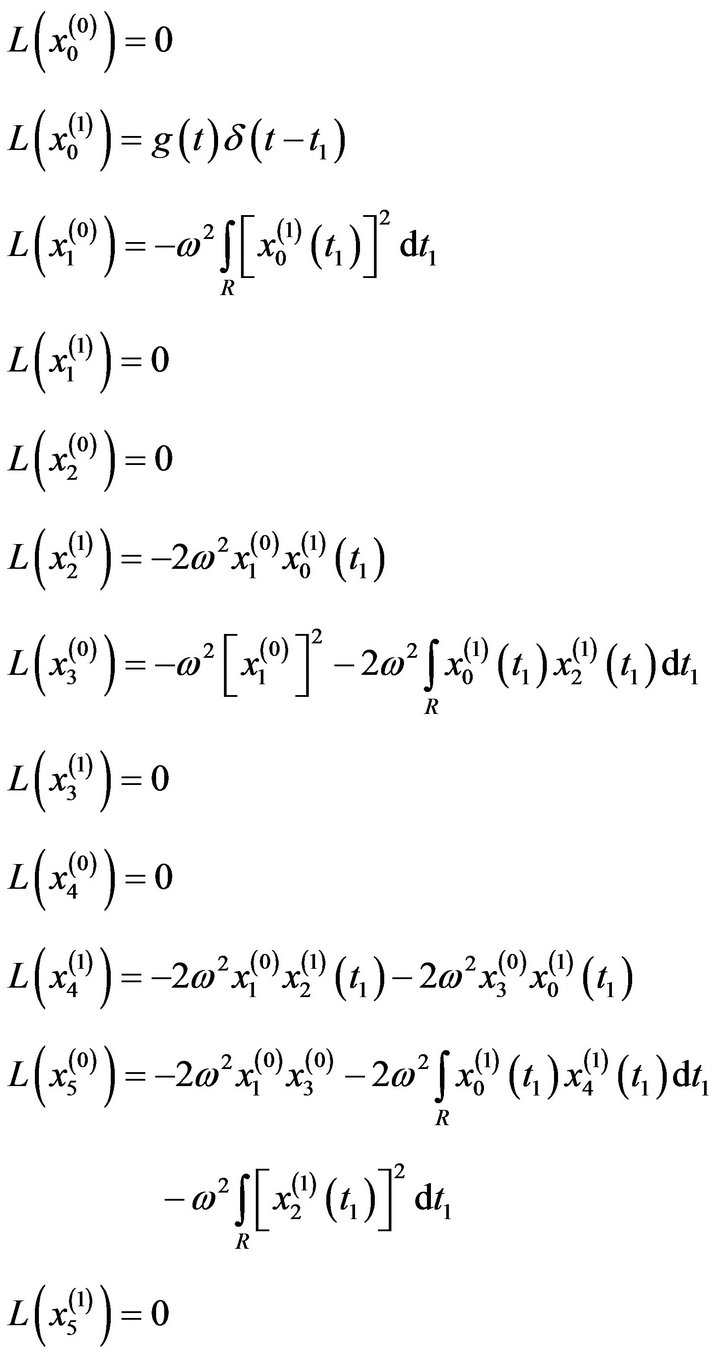
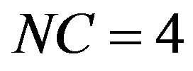
The second order  equations will be:
 :
:

 : The above equations in addition to:

 : The above equations in addition to:

 : The above equations in addition to:

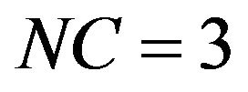
The third order  equations are:
 :
:
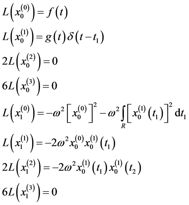
 : The above equations in addition to:

 : The above equations in addition to:

 : The above equations in addition to:


The fourth order  equations are:
 :
:

 : The above equations in addition to:
5. Results
The following output is simulated using Mathematica. The solution (11) of the model Equation (10) is used to get all kernels with the proper right hand side. The mean response and the response variance are then calculated from the kernels using Equation (9):
Figures 1 and 2 show the response mean and variance, respectively, for the case of zero initial conditions, zero deterministic exciatation and unit envelope function multiplied by the white noise. The angular frequency  and the damping ratio
 . The nonlinearity strength is changed to study its effect on the response mean and variance. As it is shown in the figures, the nonlinearity strength greatly affect the amplitudes of the mean and variance. It should not be increased after a certain value to obtain convergent solution. This value depends on the different parameters of the problem.
Also, we can notice that higher correction solutions are required with longer time intervals.
In Figures 3 and 4, the envelope function  is taken as
 . This will attenuate the effect of the white noise as the time increases. We can notice the attenuation effect on the response variance as the time increases. In this case, the variance vanishes with time and the solution becomes nearly deterministic.
In Figures 5 and 6, non-zero initial condition is considered;  and
and . The third correction mean and variance differs from the first and second corrections noticeably. This ensures the need for higher corrected WHEP solutions especially with larger values for the nonlinearity strength
![]() .
.
In Figures 7 and 8, the second order solution is simulated for different nonlinearity strengths with the first and second corrections. Higher corrected solutions will be time consuming even with multi-core machines. Mathematica automatically runs in parallel when multiple cores are available. The estimation of the response variance is more difficult than the response mean for higher corrections.
In Figures 9 and 10, the third order solution is simulated. Also, higher corrected solutions will be time con-


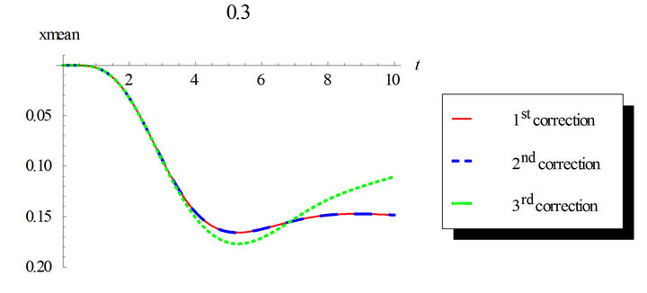

Figure 1. First order mean response for the first, second and third corrections. Comparison between the different corrections for ε = 0.3 and ε = 0.5. Case of zero initial conditions, zero deterministic force and unit envelop deterministic function multiplied by the white noise. The angular frequency  and the damping ratio
 .
.
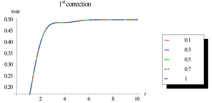


Figure 2. First order response variance for the first, second and third corrections. Comparison between the different corrections for ε = 0.3 and ε = 0.5. Case of zero initial conditions, zero deterministic force and unit envelop deterministic function multiplied by the white noise. The angular frequency  and the damping ratio
 .
.


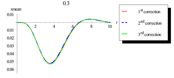

Figure 3. First order mean response for the first, second and third corrections. Comparison between the different corrections for ε = 0.3 and ε = 0.5. Case of zero initial conditions, zero deterministic force and  envelop deterministic function multiplied by the white noise. The angular frequency
  and the damping ratio
 .
.


Figure 4. First order response variance for the first, second and third corrections. Comparison between the different corrections for ε = 0.3 and ε = 0.5. Case of zero initial conditions, zero deterministic force and  envelop deterministic function multiplied by the white noise. The angular frequency
  and the damping ratio
 .
.
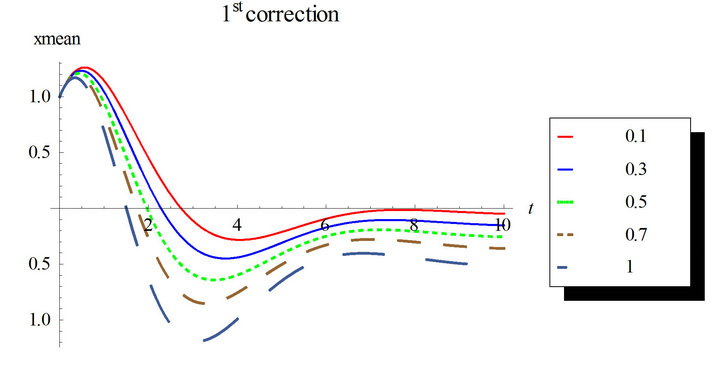


Figure 5. First order mean response for the first, second and third corrections. Comparison between the different corrections for ε = 0.3 and ε = 0.5. Case of initial conditions  and
and , zero deterministic force and unit envelop deterministic function multiplied by the white noise. The angular frequency
  and the damping ratio
 .
.


Figure 6. First order response variance for the first, second and third corrections. Comparison between the different corrections for ε = 0.3 and ε = 0.5. Case of initial conditions  and
and , zero deterministic force and unit envelop deterministic function multiplied by the white noise. The angular frequency
  and the damping ratio
 .
.

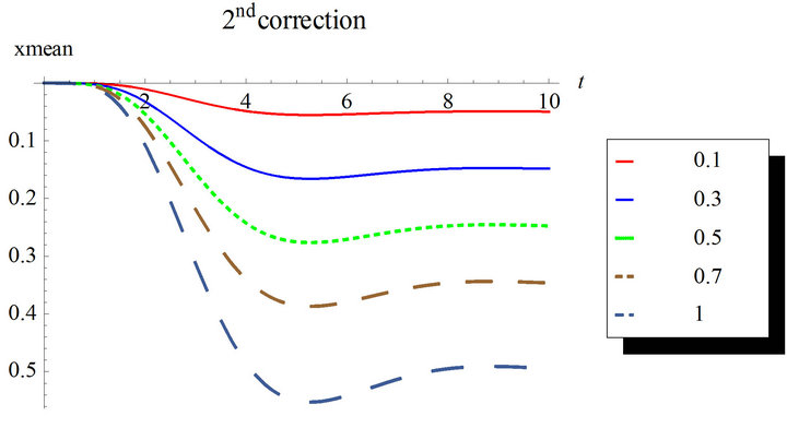
Figure 7. Second order mean response for the first and second corrections. Case of zero initial conditions, zero deterministic force and unit envelop deterministic function multiplied by the white noise. The angular frequency  and the damping ratio
 .
.
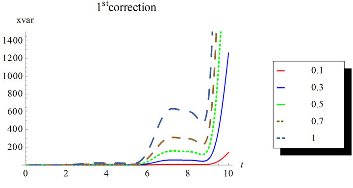

Figure 8. Second order response variance for the first and second corrections. Case of zero initial conditions, zero deterministic force and unit envelop deterministic function multiplied by the white noise. The angular frequency  and the damping ratio
 .
.


Figure 9. Third order mean response for the first and second corrections. Case of zero initial conditions, zero deterministic force and unit envelop deterministic function multiplied by the white noise. The angular frequency  and the damping ratio
 .
.


Figure 10. Third order response variance for the first and second corrections. Case of zero initial conditions, zero deterministic force and unit envelop deterministic function multiplied by the white noise. The angular frequency  and the damping ratio
 .
.
suming especially when estimating the response variance.
The fourth order first correction solution is also obtained but it is the same as the third and the second order with first corrections. Higher corrections will be more and more expensive. There is a need for an alternative method such as the numerical estimations to overcome the difficulties in using symbolic packages.
6. Conclusion
In the present paper, we investigate the mean response of the quadratic nonlinear oscillatory system subjected to nonstationary random excitation using WHEP technique. The equivalent deterministic equations have been derived up to fourth order. The corrections are considered up to the fifth correction for lower orders and second corrections for higher orders. The mean and variance are simulated using Mathematica. It is observed that the WEHP technique can be applied to study the non-Gaussian response of any random systems. Moreover, the higherorder terms of the WHE should be adopted to obtain the responses of nonlinear random systems, and the integrodifferential equations for the kernels should be calculated. There is a need for numerical estimations when higher order and higher corrections are required.
7. Acknowledgements
We should thank Prof. Magdy El-Tawil (has passed away) for motivating us to cooperate and do this work.
REFERENCES
- A. Jahedi and G. Ahmadi, “Application of Wiener-Hermite Expnasion to Nonstationary Random Vibration of a Duffing Oscillator,” Transactions of the ASME, Vol. 50, 1983, pp. 436-442.
- J. C. Cortes, J. V. Romero, M. D. Rosello and R. J. Villanueva, “Applying the Wiener-Hermite Random Technique to Study the Evolution of Excess Weight Population in the Region of Valencia (Spain),” American Journal of Computational Mathematics, Vol. 2, No. 4, 2012, pp. 274-281. doi:10.4236/ajcm.2012.24037
- W. Lue, “Wiener Chaos Expansion and Numerical Solutions of Stochastic Partial Differential Equations,” PhD Thesis, California Institute of Technology, Pasadena, 2006.
- M. A. El-Tawil, “The Application of the WHEP Technique on Partial Differential Equations,” Journal of Difference Equations and Applications, Vol. 7, No. 3, 2003, pp. 325-337.
- M. A. El-Tawil and A. S. Al-Johani, “Approximate Solution of a Mixed Nonlinear Stochastic Oscillator,” Computers & Mathematics with Applications, Vol. 58, No. 11- 12, 2009, pp. 2236-2259. doi:10.1016/j.camwa.2009.03.057
- M. A. El-Tawil and A. S. El-Johani, “On Solutions of Stochastic Oscillatory Quadratic Nonlinear Equations Using Different Techniques, A Comparison Study,” Journal of Physics: Conference Series, Vol. 96, No. 1, 2008. http://iopscience.iop.org/1742-6596/96/1/012009
- M. A. El-Tawil and A. Fareed, “Solution of Stochastic Cubic and Quintic Nonlinear Diffusion Equation Using WHEP, Pickard and HPM Methods,” Open Journal of Discrete Mathematics, Vol. 1, No. 1, 2011, pp. 6-21. doi:10.4236/ojdm.2011.11002
- M. A. El-Tawil and A. A. El-Shekhipy, “Approximations for Some Statistical Moments of the Solution Process of Stochastic Navier-Stokes Equation Using WHEP Technique,” Applied Mathematics & Information Sciences, Vol. 6, No. 3S, 2012, pp. 1095-1100.
- M. A. El-Tawil and A. A. El-Shekhipy, “Statistical Analysis of the Stochastic Solution Processes of 1-D Stochastic Navier-Stokes Equation Using WHEP Technique,” Applied Mathematical Modelling, Vol. 37, No. 8, 2013, pp. 5756-5773. doi:10.1016/j.apm.2012.08.015
- A. S. El-Johani, “Comparisons between WHEP and Homotopy Perturbation Techniques in Solving Stochastic Cubic Oscillatory Problems,” AIP Conference Proceedings, Vol. 1148, 2010, pp. 743-752. doi:10.1063/1.3225426
- N. Wiener, “Nonlinear Problems in Random Theory,” MIT Press, John Wiley, Cambridge, 1958.
- R. H. Cameron and W. T. Martin, “The Orthogonal Development of Non-Linear Functionals in Series of Fourier-Hermite Functionals,” Annals of Mathematics, Vol. 48, 1947, pp. 385-392.
- T. Imamura, W. Meecham and A. Siegel, “Symbolic Calculus of the Wiener Process and Wiener-Hermite Functionals,” Journal of Mathematical Physics, Vol. 6, No. 5, 1965, pp. 695-706.
- W. C. Meecham and D. T. Jeng, “Use of the WienerHermite Expansion for Nearly Normal Turbulence,” Journal of Fluid Mechanics, Vol. 32, 1968, pp. 225-235.
- X. Yong, X. Wei and G. Mahmoud, “On a Complex Duffing System with Random Excitation,” Chaos, Solitons and Fractals, Vol. 35, No. 1, 2008, pp. 126-132. doi:10.1016/j.chaos.2006.07.016
- P. Spanos “Stochastic Linearization in Structural Dynamics,” Applied Mechanics Reviews, Vol. 34, 1980, pp. 1-8.
- W. Q. Zhu, “Recent Developments and Applications of the Stochastic Averaging Method in Random Vibration,” Applied Mechanics Reviews, Vol. 49, No. 10, 1996, pp. 72-80. doi:10.1115/1.3101980
- E. F. Abdel-Gawad and M. A. El-Tawil, “General Stochastic Oscillatory Systems,” Applied Mathematical Modelling, Vol. 17, No. 6, 1993, pp. 329-335.
- J. Atkinson, “Eigenfunction Expansions for Randomly Excited Nonlinear Systems,” Journal of Sound and Vibration, Vol. 30, No. 2, 1973, pp. 153-172. doi:10.1016/S0022-460X(73)80110-5
- A. Bezen and F. Klebaner, “Stationary Solutions and Stability of Second Order Random Differential Equations,” Physica A, Vol. 233, No. 3-4, 1996, pp. 809-823. doi:10.1016/S0378-4371(96)00205-1
- A. Nayfeh, “Problems in Perturbation,” John Wiley & Sons, New York, 1993.
- M. A. El-Beltagy and M. A. El-Tawil, “Toward a Solution of a Class of Non-Linear Stochastic Perturbed PDEs Using Automated WHEP Algorithm,” Applied Mathematical Modelling, in Press. doi:10.1016/j.apm.2013.01.038
- MathML Website. http://www.w3.org/Math/