Journal of Environmental Protection
Vol.4 No.5(2013), Article ID:31421,14 pages DOI:10.4236/jep.2013.45055
Water Quality Assessment of River Ogun Using Multivariate Statistical Techniques
![]()
Department of Chemistry, University of Ibadan, Ibadan, Nigeria.
Email: bolaoketola@yahoo.com
Copyright © 2013 Adebola A. Oketola et al. This is an open access article distributed under the Creative Commons Attribution License, which permits unrestricted use, distribution, and reproduction in any medium, provided the original work is properly cited.
Received February 16th, 2013; revised March 19th, 2013; accepted April 7th, 2013
Keywords: Surface Water; Heavy Metals; Water Quality; PCA; CA
ABSTRACT
Variations in water quality of River Ogun around the cattle market, Isheri along Lagos-Ibadan express road were evaluated using multivariate statistical techniques such as principal component analysis (PCA) and cluster analysis (CA) to analyze the similarities or dissimilarities among the sampling points so as to identify spatial and temporal variations in water quality and sources of contamination over time. Water quality data were generated from 8 sampling points during 6 year sampling periods (i.e., 2000, 2005, 2006, 2009, 2010, and 2011). The samples were analyzed for 14 physico-chemical parameters and heavy metals such as temperature, pH, total solids (TS), total dissolved solids (TDS), suspended solids (SS), oil and grease, dissolved oxygen (DO), chemical oxygen demand (COD), Cl−1, alkalinity, total hardness (TH),  ,
,  ,
,  and heavy metals (Cd, Cu, Fe, Ni, Pb, Mn, and Zn). Three zones were differentiated based on the cluster analysis results, and implied similar water quality features. Thus, the water quality around the site may be categorized as relatively less polluted, moderately polluted and highly polluted. The PCA assisted to extract and recognize the factors responsible for water quality variations over the years. The results showed that the index which changes the quality of the water differs. The natural, inorganic and organic parameters e.g., temperature, TS, and
  etc., were the most significant parameters contributing to the variations in the water quality over the years. This shows that a parameter that can be significant in contributing to water quality in one season may less or not be significant in another. This result may be used to reduce the number of samples analyzed both in space and time, without much loss of information. This will assist the decision makers in identifying priorities to improve water quality that has deteriorated due to pollution from various anthropogenic activities.
1. Introduction
Water of adequate quantity and quality is essential for sustainable development [1]. Water quality performs important role in health of human, animals and plants [2,3]. Water quality is the critical factor that influences human health as well as the quantity and quality of grain production in semi-humid and semi-arid area [4]. Water pollution is harmful not only to fish breeding and agricultural products but also to public health in surrounding areas. Of the pollutants, heavy metals can endanger health by being incorporated into food chain. Heavy metals are not biodegradable and tend to accumulate in the sediments of water ways in association with organic and inorganic matter in the sediment [5]. Excessive nutrients can lead to water eutrophication, causing a hypoxia environment, the reductions of species diversity and microbial growth, mortality of benthic communities, and stress in fishery resources [6]. Human activities are a major factor determining the quality of surface and ground water through atmospheric pollution, effluent discharges, use of agricultural chemicals, eroded soils and land use [7]. These land use changes increase the amount of impervious surface resulting in storm runoff events that negatively affect stream ecosystems and water quality [8]. Rivers in water sheds with substantial agricultural and urban land use experience increased inputs and varying compositions of organic matter [9] and excessive concentrations of phosphorus and other nutrients from fertilizer application and watershed releases [10].
The quality of surface water within a region is governed by both natural processes (such as precipitation rate, weathering processes and soil erosion, hydrological processes; physical, chemical and biological processes) [1,2] and anthropogenic effects (such as urban, industrial and agricultural activities and the human exploitation of water resources) [11,12]. Seasonal variation in precipitation, surface run-off, groundwater flow, interception and abstraction strongly affect river discharge and consequently the concentrations of pollutants in river water [2]. The impact of agricultural activities on water quality is gaining increasing attention [13]. Studies have indicated that many rivers/streams particularly in developing countries are heavily polluted due to industrial and municipal wastewater discharges, as well as agricultural runoff [14- 17].
The multidimensional data analysis methods are becoming very popular in environmental studies dealing with measurement and monitoring. The most common multidimensional data analysis methods used are cluster analysis (CA), factor analysis/principal component analysis (FA/PCA), which have been used to identify important components/sources that explain the variations in water quality and influence the water system [13]. The application of different multivariate statistical techniques such as CA, PCA, factor analysis (FA) and discriminant analysis (DA) facilitates the interpretation of complex data matrices to better understand the water quality and ecological status of studied systems [18]. Usually, CA is used to reveal specific links between sampling points, while FA/PCA is used to identify the ecological aspects of pollutants on environmental systems [13,14]. Principal components are nothing more than the eigenvectors of a variance-covariance or a correlation matrix of the original data matrix. By themselves they may provide significant insight into the structure of the matrix not available at first glance. Typically, the raw data matrix can be reduced to two or three principal component loadings that account for the majority of the variance. The first principal component loading explains the most variance and each subsequent component explains progressively less [19]. As a result, a small number of factors usually accounts for approximately the same amount of information as the much larger set of the original observations do. PCA can be applied to a set of water quality variables to discover the variables that form coherent subsets that are relatively independent of one another. Cluster analysis comprises of multivariate methods which are used to find true groups of data. In clustering, the objects are grouped such that similar objects fall into the same class [19]. This multivariate treatment of environmental data is widely successfully used to interpret relationships among variables so that the environmental system could be better managed [19,20].
The aim of this study was to determine 14 physicochemical parameters and heavy metals in River Ogun water around the cattle market, Isheri along Lagos-Ibadan express road. The data obtained was subjected to the multivariate statistical methods (CA and PCA) to evaluate information about similarities and dissimilarities between sampling points, to recognize water quality variables that causes variations and the effect of pollution sources on the water quality in general.
2. Materials and Methods
2.1. Description of the Study Area
River Ogun is one of the rivers in the south-western part of Nigeria which covers a total area of about 22.4 Km2. It transverses through Ibarapa, Iseyin, Abeokuta, Owode, Ikorodu, and Ifo local government areas before finally discharging into the Lagos Lagoon. This site has become a place of interest considering its constant and continuous pollution owing to the fact that it serves as a focal point of some commercial activities in the ever growing cattle market around the basin. Figure 1 shows the map of the study area while the sampling point’s location is presented in Table 1.
2.2. Sample Collection
Water samples were collected from 8 sampling points in 2000, 2005, 2006, 2009, 2010 and 2011. Grab samples were collected by dipping already cleaned sample containers gently into the water at different points. At each sampling points, five samples were collected and mixed together to form a composite. The collected samples were stored in a cooler containing ice, delivered on the same day to the laboratory where they were refrigerated until analysis.
2.3. Analytical Methods
Refrigerated samples were allowed to attain room temperature prior to analysis. Temperature and pH were measured on site with a mercury thermometer (range 0˚ to 100˚C) and a digital portable pH meter, respectively. Total dissolved solids (TDS) and oil and grease (OLG) were determined by gravimetry; total hardness (TH), alkalinity (ALK), dissolved oxygen (DO) (Winkler’s method), chemical oxygen demand (COD) (open reflux), chloride (Cl−) (silver nitrate method) were determined by titrimetry according to standard methods [21,22]; sulphate ( ) by turbidimetry using PYE UNICAM SP -200 spectrophotometer and phosphate (
 ) using ammonium molybdate and potassium antimonyl tartrate reagents. Nitrate (
 ) was determined by phenoldisulphonic acid method [23]. Acidified samples were digested with concentrated HNO3 acid for heavy metal determination prior to analysis using atomic absorption spectrophotometer, Buck Scientific model 200A. Blanks and duplicate determination were carried out to check

Figure 1. Map of the study area showing the sampling points.
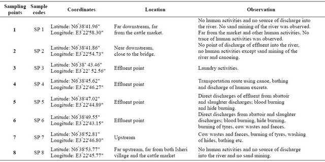
Table 1. Sampling points, sample codes, location and observation.
and remove possible errors. All instruments used were calibrated with appropriate standard solutions prior to sample analysis and measurement.
2.4. Statistical Analysis
The statistical software package SPSS 15 window was used for the descriptive analysis, correlation coefficient and multivariate statistical analysis of the data.
2.4.1. Principal Component Analysis (PCA)
PCA provides information on the most meaningful parameters which describe the whole data set interpretation, data reduction and summarize the statistical correlation among constituents in the water with minimal loss of original information [24,25].
In this study, PCA of the normalized variables were executed to extract significant principal components (PCs) and to further reduce the contribution of variables with minor significance; these PCs were subjected to varimax rotation generating factors [26]. PCs were defined according to the criterion that only factors that account for variance greater than 1 (eigenvalue-one criterion) should be included. The rationale for this is that any component should account for more variance than any single variable in the standardized test score space [13]. Hence, PCA was applied using varimax rotation with Kaiser Normalization. By extracting the eigenvalues from the correlation matrix, the number of significant factors and the percent of variance explained by each of them were calculated.
2.4.2. Cluster Analysis (CA)
Cluster analysis is a group of multivariate technique whose primary aim is to assemble objects based on the characteristics they possess [26]. In clustering, the objects are grouped such that similar objects fall into the same class [27]. According to [28], cluster analysis is a multivariate technique used to find homogeneous groups with respect to certain properties. Hierarchical clustering joins the most similar observations and successively the next most similar observations. The levels of similarity at which observations are merged are used to construct a dendrogram. To perform CA, an agglomerative hierarchical clustering was developed using a combination of the Ward’s linkage method and squared Euclidean distances as a measure of similarity [29]. The hierarchical method of cluster analysis used in this study has the advantage of not demanding any prior knowledge of the number of clusters, while the non-hierarchical method does [30]. Cluster analysis groups data and objects based on information found in the data that describes the objects and their relationships. The reason for this is to ensure that the objects within a group are similar (or related) to one another and different from (or unrelated to) the objects in other groups. The greater the similarity (homogeneity) within a group and the greater the difference between groups is, the better or more distinct the clustering [31] will be.
3. Results and Discussion
3.1. Current Water Quality
The results of the physico-chemical parameters and the descriptive statistics of the samples collected at different points around the cattle market are presented in Table 2 while Table 3 shows the correlation coefficient. The pH

Table 2. Mean concentration and general descriptive statistics of the physico-chemical parameters of River Ogun around the market (Present study).

Table 3. Correlation coefficient of physico-chemical parameters and heavy metals of river Ogun around the market.
*Correlation is significant at the 0.05 level (2-tailed). **Correlation is significant at the 0.01 level (2-tailed).
values ranged from 6.60 - 6.73 with a mean value of 6.68± 0.04 which indicates that the river is slightly acidic. There is strong correlation at p < 0.05 between pH and COD (r = 0.71). The temperature ranged from 28˚C - 32˚C with a mean value of 30.3˚C ±1.3˚C. However, highest temperature of 32˚C was recorded at SP 5 which was the point of direct hot effluent discharge into the river, blood cooking and hide burning. The concentration of oil and grease ranged from 120 - 3400 mg/L with a mean concentration of 1000 ± 1100 mg/L. There is very strong correlation at p < 0.01 between oil and grease and SS (r = 0.94), nitrate (r = 0.90), phosphate (r = 0.89), sulphate (r = 0.88), and TS (r = 0.84) (Table 3). The concentration of alkalinity ranged from 105 - 146 mg/L with a mean value of 122 ± 13 mg/L. The quantity of waste in different phases of a natural aquatic system is reflected by the level of hardness, alkalinity, free CO2 and other physico-chemical parameters [32]. There is strong and significant correlation at p < 0.01 between alkalinity and sulphate (r = 0.84). Total hardness concentration obtained in this study ranged from 43.6 - 56.6 mg/L with a mean concentration of 51.3 ± 4.7 mg/L. Based on classification [33], River Ogun water is moderately hard, thereby limiting its use for some domestic purposes, such as washing. The water could be a good source for livestock weathering. In addition, it cannot be used for industrial purposes as hard water forms clogs that can block boilers and pipes [34], thus necessitating its treatment before use for certain industrial applications. Also, the water is not good for irrigation due to high level of cadmium and manganese based on water quality criteria by Food and Agriculture Organization [35] and Federal Environmental Protection Agency [36].
The range and the mean concentration of TS of River Ogun around the market are 220 - 1460 mg/L and 803 ± 450 mg/L, respectively. The concentrations increased from the far downstream up to the effluent discharge points while a gradual decrease in concentration was observed at the upstream. According to [37], total solids depend on base flow, run-off, and anthropogenic sources such as industrial and municipal wastes as well as agricultural wastes. Hence, the high concentrations at the effluent points could be attributed to anthropogenic sources from human activities, eroded soil particles, road surface degradation and runoffs, degradation of automobile tyres, effluent discharge along side with animal waste disposal. The TS obtained from this study was higher than those obtained from previous studies [38]. There is strong and significant correlation at p < 0.01 between TS and TDS (r = 0.997), phosphate (r = 0.93), nitrate (r = 0.92), COD (r = 0.87), SS (r = 0.87), and oil and grease (r = 0.84). TDS ranged from 120 - 1240 mg/L with a mean concentration of 660 ± 400 mg/L. TDS comprises of inorganic salts (principally calcium, magnesium, potassium, sodium, bicarbonates, chlorides and sulphates) and small amount of organic matter that are dissolved in water. TDS in water originate from natural sources, sewage, urban runoff and industrial wastewater [39]. Concentration of TDS in water varies considerably in different geological regions owing to differences in the solubility of minerals. There is very strong and significant correlation at p < 0.01 between TDS and TS (r = 0.99), phosphate (r = 0.91), nitrate (r = 0.90), and COD (r = 0.86) (Table 3). The range and mean concentration of SS are 80 - 260 mg/L and 143 ± 58 mg/L, respectively. The concentration of SS obtained in this study was higher than those from the previous studies [38]. There is significant and strong correlation at p < 0.01 between SS and oil and grease (r = 0.94), phosphate (r = 0.93), nitrate (r = 0.92), COD (r = 0.87), and sulphate (r = 0.84).
The range and mean concentration of DO are 2.90 - 5.08 mg/L and 4.04 ± 0.81 mg/L, respectively. The decrease in DO values noticed from one sampling point to another could be attributed to the fact that as the river flows along its course, it carries soil and partially dissolved and undissolved organic and inorganic matters which are oxidized by the DO present in the water thereby leading to a decrease in the DO. The low DO values could also be as a result of the degradation of cattle waste, cattle feed and hot discharges into the river which are oxygen demanding [40]. In addition, as water flows through towns and cities, different oxygen demanding substances are discharged into the water [41]. Excessive algae and plant growth can lead to depletion of dissolved oxygen, which adversely affects organisms population. There is very strong and significant correlation at p < 0.01 between DO and Cu (r = 0.92). The oxygen content of a water body is mainly controlled by the decay of organic substances, the oxidation of the nitrogen compounds and the photosynthetic aeration of the water by plants and oxygen demand by sediments. Reduced oxygen levels can kill fish and other aquatic life in the river. The range and mean concentration of chemical oxygen demand are 98 - 300 mg/L and 197 ± 78 mg/L, respectively. The presence of high biodegradable and non-biodegradable matters as well as exposure of sediment in the river which may have accumulated organic and inorganic matters over a period of time could account for this trend. There is very strong and significant correlation at p < 0.01 between COD and phosphate (r = 0.96), TS (r = 0.87), SS (r = 0.87), TDS (r = 0.86), and sulphate (r = 0.85) (Table 3).
The concentration of chloride ranged between 43.6 - 55.1 mg/L with a mean concentration of 48.7 ± 4.4 mg/L. Chloride in drinking-water originates from natural sources, sewage, industrial effluents and urban runoff. Excessive chloride concentration increases the rate of corrosion of metals in the water distribution system and depending on the alkalinity of the water; this can lead to increased concentrations of metals in the supply [39]. Chloride concentration in excess of about 250 mg/L can give rise to detectable taste in water. The range of sulphate concentration in the water was 2.88 - 34.8 mg/L with a mean concentration of 14.5 ± 10 mg/L. This could be attributed to the fact that sulphate occur naturally in numerous minerals and are used principally in the chemical industry. They are discharged into water body from industrial wastewater and through atmospheric deposition [39]. There is strong and significant correlation at p < 0.01 between sulphate and oil and grease (r = 0.88), phosphate (r = 0.85), COD (r = 0.85), SS (r = 0.84), and alkalinity (r = 0.84).
The concentration of nitrate around the market ranged from 6.51 - 16.5 mg/L with a mean concentration of 10.4 ± 3.7 mg/L. This was also higher than those obtained from previous studies [38]. This increase could be accounted for by the continuous discharge of nitrogenous compounds in animal waste, agricultural runoff, oxides of nitrogen emitted during burning of bones, horns and hides etc. Nitrates are high oxide form of nitrogenous compounds and are usually present in surface water. It is the end product of aerobic decomposition of organic nitrogenous matter present in animal waste. Also, atmospheric nitrogen is washed down by rain into streams, lakes, rivers, and coastal waters which in turns lead to an increase in nitrate level and then contributes to algal blooms that deprive fish and other aquatic organisms of oxygen [42]. The accumulation of excess nutrients over a period of time could also lead to eutrophication and the loss of aquatic and other microorganisms in the river. The primary health concern regarding high levels of nitrate and nitrite in potable water is the formation of methaemoglobinaemia, so-called “blue-baby syndrome”. Nitrate is reduced to nitrite in the stomach of infants. This reduction of nitrate to nitrite by gastric bacteria is also higher in infants because of low gastric acidity. The nitrate concentration in groundwater and surface water is normally low but can reach high level as a result of leaching or run-off from agricultural land or contamination from human or animal wastes [39]. There is very strong and significant correlation at p < 0.01 between nitrate and phosphate (r = 0.95), SS (r = 0.92), TS (r = 0.92), TDS (r = 0.90), and oil and grease (r = 0.90). Phosphate concentration ranged between 1.51 - 4.40 mg/L with a mean concentration of 2.75 ± 1.0 mg/L (Table 3). The presence of water hyacinths on the surface of the river around some sampling points could be attributed to increase in nutrient in the water. Nitrate and phosphate are nutrients very essential for plant growth. However, high concentrations tends to pose more harm on the water body as they can lead to algal growth commonly refer to as algal bloom. It has been reported that excess concentration of phosphorus of 0.015 mg/L and nitrogen concentration of about 0.3 mg/L are sufficient to cause algal bloom [37].
Eutrophication could adversely affect the use of rivers and dams for recreational purposes as the covering of large areas by water hyacinth could cause unsightly and malodorous scum, which could lead to the growth of algae as well as the release of toxic substances into the water body. The first step to eutrophication is the addition of nutrients to the water, increase in nutrient causes algae bloom, as the algae bloom progresses, the algae begin to die, and organic material accumulates on the bottom of the river. This material supports a boom in the decomposer population and the decomposers rapidly rob the river of its oxygen, suffocating most other organisms in the process. Eutrophication leads to an increase in the treatment cost of potable water as it lead to filter clogging in water treatment plants. Also, high nutrient concentrations interfere with recreation and aesthetic enjoyment of water resources by causing reduced water clarity, odour and blooms of toxic and nontoxic organisms [22]. There is very strong and significant correlation at p < 0.01 between phosphate and COD (r = 0.96), nitrate (r = 0.95), SS (r = 0.93), TS (r = 0.93), TDS (r = 0.91), oil and grease (r = 0.89), and sulphate (r = 0.85).
The concentration of Cd ranged from ND - 0.03 mg/L with a mean concentration of 0.01 ± 0.0 mg/L (Table 4). Cadmium is released into the environment in wastewater and diffuse pollution is caused by contamination from fertilizer, local air pollution and leachate from landfill or dumpsite [39]. Contamination in drinking-water may be caused by impurities in the zinc of galvanized pipes and solders and some metal fittings. Cadmium accumulates primarily in the kidneys and has a long biological halflife of 10 - 35 years in humans. Hence, kidney is the main target organ for cadmium toxicity. Therefore, chronic exposure by accumulation of cadmium in the environment must, however, be considered under conditions of long-term irrigation water use and soil type. There is very strong and significant correlation at p < 0.01 between Cd and Pb (r = 1.0). Concentration of Cu ranged from ND - 0.01 mg/L with a mean concentration of 0.01 ± 0.0 mg/L. Copper is both an essential nutrient and a drinking-water contaminant with many commercial uses. It is used to make pipes, valves and fittings and is present in alloys and coatings [39]. Copper sulphate pentahydrate is sometimes added to surface water for the control of algae. Copper concentration in drinking-water varies widely with the primary source most often being the corrosion of interior copper plumbing. Level in running or fully flushed water tends to be low, whereas those in standing or partially flushed water sources are more variable and can be substantially higher (frequently > 1 mg/L). Copper concentrations in treated water often
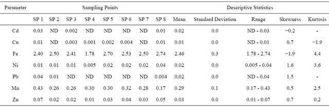
Table 4. Mean concentration and the descriptive statistics of heavy metals of River Ogun water around the market (Present study).
increase during distribution, especially in systems with an acid pH or high-carbonate waters with an alkaline pH [39]. There is very strong and significant correlation at p < 0.01 between Cu and Pb (r = 1.0), Zn (r = 0.95), DO (r = 0.92).
The concentration of Fe in River Ogun water around the cattle market ranged from 1.78 - 2.74 mg/L with a mean concentration of 2.46 ± 0.3 mg/L. Corrosive materials contribute significantly to the amount of iron in water. Iron is one of the most abundant metals in the earth’s crust. It is found in natural fresh waters at levels ranging from 0.5 to 50 mg/L. Iron is an essential element in human nutrition, however, estimates of the minimum daily requirement for iron depend on age, sex, physiological status and iron bioavailability and range from about 10 to 50 mg/day [39]. Iron stains laundry and plumbing fixtures at levels above 0.3 mg/L. There is usually no noticeable taste at iron concentrations below 0.3 mg/L, and concentrations of 1 - 3 mg/L can be acceptable for people drinking anaerobic well water. The concentration of Ni ranged from 0.01 - 0.04 mg/L with a mean concentration of 0.02 ± 0.0 mg/L. Food is the dominant source of nickel exposure in the non-smoking, non-occupationally exposed population while water is generally a minor contributor to the total daily oral intake [39]. There is moderate correlation at p < 0.01 between Ni and Fe (r = 0.59) and Zn (r = 0.55). The concentration of Pb in River Ogun water obtained in this study ranged from ND - 0.04 mg/L with a mean concentration of 0.02 ± 0.0 mg/L. Lead is one of the significant toxic metals. There is very strong and significant correlation at p < 0.01 between Pb and Cu (r = 1.0). The concentration of Mn ranged from 0.17 - 0.43 mg/L with a mean concentration of 0.29 ± 0.1 mg/L. Zn concentration ranged from 0.01 - 0.07 mg/L with a mean concentration of 0.03 ± 0.0 mg/L. Zinc is associated with human activities such as the use of chemicals and zinc based fertilizers [43]. There is very strong and significant correlation at p < 0.01 between Zn and Cu (r = 0.95) (Table 3).
3.2. Statistical Analysis
Principal Component Analysis (PCA)
In order to evaluate the most significant parameters in water quality assessment, the analysis was performed using PCA methodology. PCA was executed in this study for the 21 variables from 8 different sampling points in the 6 years (2000, 2005, 2006, 2009, 2010 and 2011) of monitoring the water quality in order to identify important water quality parameters.
An eigenvalue gives a measure of the significance of the factor and factors with the highest eigenvalues are the most significant. Eigenvalues of 1.0 or greater are considered significant [26]. Classification of principal components is thus “strong”, “moderate” and “weak”, corresponding to absolute loading values of >0.75, 0.75 - 0.50 and 0.50 - 0.30, respectively [20]. Tables 5 and 6 summarizes the PCA including the loadings, eigenvalues of each PCs, total variance explained as well as the cumulative variance and strong loading values highlighted. The PCA of the data obtained in 2000 (Table 5), showed six PCs which explained 96.7% of the total variance. The first PC explained 33.0% of the total variance and was best represented by COD, TH, Cd, Cu, Fe, Ni, Pb and Mn. PC 2 was dominated by temperature, pH, SS, alkalinity, TH and Cd, accounted for 17.4% of the total variance. PC 3 explained 15.2% of the total variance and loaded heavily on oil and grease, DO, sulphate and Mn. PC 4 was loaded primarily by TS and TDS, accounting for 13.8% while additional, 8.96% of the total variance was explained in PC 5 which was contributed by pH, nitrate and Zn. PC 6 was responsible for 8.55% of the total variance and was best represented by chloride and phosphate.
In the PCA of data obtained in 2005 [44], five components were extracted which explained 93.8% of the
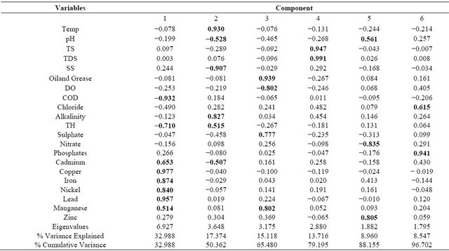
Table 5. PCA of water quality parameters of River Ogun in 2000.
Note: Extraction Method: Principal Component Analysis; Rotation Method: Varimax with Kaiser Normalization; Bold figures indicate absolute values >0.5 of parameters with strong loading value.

Table 6. PCA of water quality parameters of River Ogun in 2011.
Note: Extraction Method: Principal Component Analysis; Rotation Method: Varimax with Kaiser Normalization; Bold figures indicate absolute values >0.5 of parameters with strong loading value.
total variance. PC 1 explained 32.3% of the variance and loaded heavily on temperature, pH, TS, TDS, SS and sulphate. PC 2 was loaded primarily by DO, alkalinity, TH, nitrate and Fe, which accounted for 29.7% of the total variance. PC 3 was responsible for 15.4% of the variance and was best represented by oil and grease, chloride, alkalinity and TH. PC 4 explained 8.73% of the total variance and was best represented by temperature, COD and phosphate. However, additional 7.73% of the variance was explained in PC 5 and loaded heavily on Cu and Zn. The PCA of data obtained in 2006 [45] also showed that six PCs were extracted which explained 96.6% of the total variance. The first PC explained 35.6% of the variance and was best represented by temperature, TS, TDS, TH, sulphate and nitrate. PC 2 was dominated by DO, COD, nitrate and phosphate which accounted for 25.7% of the total variance. PC 3 explained 12.6% of the total variance and loaded heavily on SS, oil and grease and Zn. PC 4 was loaded primarily by pH and Cd which accounted for 9.49% of the variance. Additional 6.77% of the total variance was explained by PC 5 and was contributed by chloride and alkalinity while PC 6 was responsible for 6.39% of the variance and was best represented by oil and grease and Ni.
Also, the PCA of data obtained in 2009 [46] extracted six PCs which accounted for 93.0% of the total variance. PC 1 explained 33.8% of the total variance and loaded heavily on temperature, TS, TDS, DO, COD, TH and Ni. PC 2 was loaded primarily by pH, oil and grease, alkalinity, nitrate and Mn which was 17.7% of the variance. PC 3 was responsible for 13.5% of the total variance and was best represented by TS, SS, sulphate and Cu. PC 4 explained 12.6% of the variance and was best represented by TH, Cd and Pb. Additional 9.39% of the total variance was explained in PC 5 and loaded heavily on Fe, Mn and Zn. However, PC 6 was responsible for 6.09% of the variance and was best represented by chloride and phosphate. Furthermore, the PCA of data obtained in 2010 [47] extracted five components which explained 92.2% of the total variance. PC 1 explained 30.4% of the total variance and was best represented by temperature, TS, TDS, SS, alkalinity, nitrate and Ni. PC 2 was dominated by pH, oil and grease, COD, sulphate, Cd, Cu and Fe which accounted for 26.3% of the variance. PC 3 explained 15.9% of the variance and loaded heavily on TH, Pb, Mn and Zn. PC 4 was loaded primarily by pH, DO and phosphate, accounted for 9.49% of the variance while PC 5 was responsible for 8.19% of the total variance and was best represented by pH, COD, chloride and nitrate.
Finally, the PCA of the present study (Table 6) extracted four components which accounted for 91.2% of the total variance. PC 1 explained 49.1% of the total variance and loaded heavily on TS, TDS, SS, oil and grease, DO, COD, chloride, alkalinity, sulphate, nitrate and phosphate. PC 2 was loaded primarily by temperature, Cd, Cu, Pb, Mn and Zn, accounted for 19.6% of the variance. PC 3 was responsible for 15.2% of the total variance and was best represented by chloride, TH, Fe and Ni. PC 4 explained 7.28% of the variance and was best represented by pH, alkalinity, sulphate, Cd and Cu. The most significant water quality parameters that contribute to variations in the quality of River Ogun water are presented in Table 7. Phosphate and DO were the most significant parameters contributing to the variation in water quality in all the years studied. COD, TDS, TSS, SS and oil and grease with strong loading are the most important parameters in water quality variations for five years out of the six years studied. Discharge of effluent from the slaughter houses, river sand mining and other activities in the market causes considerable pollution. The temperature with strong loadings is the most significant parameter which contributed to variation in water quality in all the years and it represents the impacts of the discharge mostly hot as most of the sampling was done during the wet season when ambient temperature is believed to be lower. There is limited access to the water during the dry season. This is due to very low water volume and the presence of water hyacinth across the water surface which hinders movement on the water surface.
3.3. Cluster Analysis (CA)
Different sampling stations in a river can be grouped into clusters of similar water quality features. When cluster analytical technique is used, it is possible to plan for coming/future events, optimum sampling strategy that can lessen the number of sampling stations and the affiliated recurring costs. It is usually used if a visual summary of the intra-relationship amongst variation parameters can lead to a better understanding of the governing factors in a studied system. Figures 2 and 3 show the dendrogram output using the Ward’s linkage method and square Euclidean distances. The clustering procedure generated three groups in a very convincing way, as the points in these groups have similar characteristic features. Clusters 1, 2 and 3 corresponds to relatively low pollution, moderate pollution and high pollution regions of the river, respectively. The CA of data obtained in 2000 (Figure 2) displayed three clusters. Cluster 1 (Sampling points 1, 6, 4, 2 and 3), Cluster 2 (Sampling points 8 and 9) and Cluster 3 (Sampling points 5 and 7), corresponds to relatively low pollution, moderate pollution and high pollution regions, respectively. In Cluster 1 which comprises relatively less polluted sites, the sampling points that formed this cluster were far from the cattle market and discharge of effluent into the river. However,
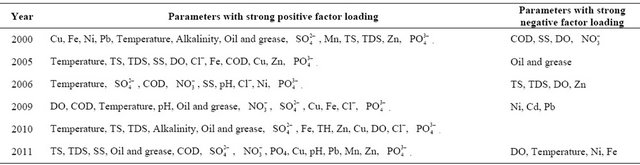
Table 7. The most significant parameters.
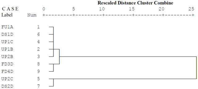
Figure 2. Dendrogram of cluster analysis of water quality parameters of River Ogun in 2000.
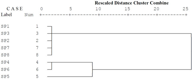
Figure 3. Dendrogram of cluster analysis of water quality parameters of River Ogun in 2011.
a dumpsite was observed at the river bank close to two of the sampling points (3 and 4). Cluster 2 corresponds to the moderately polluted sites. These sampling points receive pollution from river sand mining and domestic activities from a village not too far from the market. Two sampling points (5 and 7) of the river formed cluster 3 which are the most polluted sites. These sites were around the cattle market and close to the express road.
The data obtained in 2005 [44] also displayed 3 clusters. Cluster 1 includes sampling points 3, 5, 2, 4 and 7 which corresponds to relatively less polluted sites. Houses and domestic activities and public latrine, were observed very close to these sampling points. Points 1 and 6 formed cluster 2 which comprises of the moderately polluted site. Accounting for the extent of pollution is the presence of water hyacinth, indicating the possibility of excess nutrient from farming and fishing activities as well as sand mining around these points. Point 8 formed cluster 3 which is the most polluted site. This sampling point was around human settlement, transportation by means of canoe and sand mining activities characterized this region. The data obtained in 2006 [45], however, displayed 3 clusters with points 5, 6, 7 and 8 forming cluster 1 which comprise of relatively less polluted site. Less human activities except sand mining, vehicular emission, laundry activities and bathing were activities around these points. Point 4 formed cluster 2 which corresponds to moderately polluted site which was characterised by the discharge of domestic wastewater. Cluster 3 is made up of points 2, 3 and 1, which correspond to points experiencing high pollution. This could be attributed to the discharge of wastewater and untreated sewage as well as the discharge of cow waste and animal faeces. Also, flourishing growth of water hyacinth was seen on the river around sampling point 3 and brick making was observed at sampling point 2. The data obtained in 2009 [46] gave 3 clusters with cluster 1 comprises of points 3, 6, and 7; cluster 2 comprises of points 1, 2, 5 and 4 while cluster 3 is made up of points 8 and 9. These correspond to relatively low pollution, moderate pollution and high pollution regions, respectively. Points 3, 6 and 7 in cluster 1 are sampling points which were reasonably far from the cattle market and direct points of waste or wastewater discharge from the abattoir. Cluster 2 which is moderately polluted site were points receiving pollution from agricultural, river sand mining and fishing activities. Points 8 and 9 formed cluster 3 which was the most polluted site. Close to these points were major effluent channels from the slaughter slab and disposal of dead animal in the river.
Three clusters were also generated from the data obtained in 2010 [47]. Points 4, 6, 7, 5 and 8 formed cluster 1 which comprises relatively less polluted region. This could be attributed to the presence of little or no human activities around sampling points 7 and 8 while the burning of tyres was noticed around point 6. Points 4 and 5 were characterized by hide burning. Points 1 and 2 formed cluster 2 which corresponds to moderately polluted region. These points were close to the cattle market and other activities such as sand mining while point 3 formed cluster 3. This corresponds to the sampling point experiencing high pollution. The pollution experienced at this point could be traced to the various activities from the cattle market (abattoir and the slaughter houses). Animal blood from the slaughter slab, slaughter discharges and waste from burnt hide were discharged into the river around this point. There was the presence of water hyacinth around this point. In the present study (Figure 3), points 1, 3, 2, 7 and 8 formed cluster 1 which comprises relatively less polluted site. This could be attributed to the fact that little or no human activities were taking place at points 1, 2 and 8 while points 3 and 7 were characterized by laundry activities and washing of hides. Cluster 2 is made up of sampling points 4 and 6 which correspond to moderately polluted site. These points were the effluent discharge points from bathing and discharge of human excreta as well as direct discharge from abattoir, blood burning and hide burning. Sampling point 5 formed cluster 3 which is the most polluted sampling region on the river. This was an effluent discharge point of animal blood from abattoir, blood burning, and hides burning.
It was observed in all the years, however, that sampling points with similar features and human activities were consistently classified as either moderately or highly polluted regions. The most polluted region is points around the cattle market close to the abattoir. The results obtained from CA indicate that CA technique is useful in the classification of the regions of surface water into different categories such as relatively less pollutedmoderately polluted and highly polluted region depending on the extent of pollution. This implies that for rapid assessment of water quality, only one site in each cluster may serve as good site in spatial assessment of the water quality of the whole network.
4. Conclusion
In this study, multivariate statistical techniques were used to evaluate the variation in the surface water quality of River Ogun around the cattle market, Isheri, along Lagos—Ibadan express road. The results of PCA aided the extraction and recognition of the factors/parameters responsible for water quality variation in all the years. Phosphate, nitrate, oil and grease, TS, TDS, DO, COD, oil and grease and Cu were the significant parameters contributing to the water quality variation of the river while phosphate and DO were the most significant parameters that affected the water quality in all the years studied. PCA evinced that in temporal variation, a parameter that can be significant in contributing to water quality variation in a year may be less significant in another year. It helped to identify the parameters that always or frequently lead to the variation of the water. In addition, it could help provide a guideline for selecting the priorities of possible preventive measures in the proper management of this surface water by giving priority to minimizing the parameters identified as means of improving the water quality. CA was used in the spatial classification of water quality variation of the river. CA assisted in grouping all the sampling points into three clusters of similar water quality features. This classified the whole river into three zones of relatively less polluted, moderately polluted and highly polluted regions. The sampling points around the abattoir were the most polluted all year round. From this classification, it is possible to plan for optimum sampling strategy that can reduce the number of sampling points during assessment and the affiliated recurring cost during environmental monitoring plans of the river. Hence, the number of sampling points and the respective cost in future surface water quality monitoring plans can be lessen. This will assist the decision makers in identifying priorities to improve water quality that has deteriorated due to pollution from various anthropogenic activities.
5. Acknowledgements
The efforts and contribution of O. A. Aramide, O. G. Babalola, R. O. Owoade and A. O. Uzoh, are acknowledged.
REFERENCES
- B. Khalil and T. M. B. Ouarda, “Statistical Approaches Used to Assess and Redesign Surface Water Quality Monitoring Networks,” Journal of Environmental Monitoring, Vol. 11, No. 11, 2009, pp. 1915-1929. doi:10.1039/b909521g
- H. Pejman, G. R. Nabi Bidhendi, A. R. Karbassi, N. Mehrdadi and M. Esmaeili Bidhendi, “Evaluation of Spatial and Seasonal Variations in Surface Water Quality using Multivariate Statistical Techniques,” International Journal of Environmental Science and Technology, Vol. 6, No. 3, 2009, pp. 467-476.
- Y. Zhao, X. H. Xia, Z. F. Yang and F. Wang, “Assessment of Water Quality in Baiyangdian Lake Using Multivariate Statistical Techniques,” Procedia Environmental Sciences, Vol. 13, 2012, pp. 1213-1226. doi:10.1016/j.proenv.2012.01.115
- B. Zhang, X. Song, Y. Zhang, D. Han, C. Tang, Y. Yu and Y. Ma, “Hydrochemical Characteristics and Water Quality Assessment of Surface Water and Groundwater in Songnen Plain, Northeast China,” Water Research, Vol. 46, No. 8, 2012, pp. 2737-2748. doi:10.1016/j.watres.2012.02.033
- N. T. L. Huong, M. Ohtsubo, L. Li, T. Higashi and M. Kanayama, “Assessment of the Water Quality of Two Rivers in Hanoi City and Its Suitability for Irrigation Water,” Paddy Water Environment, Vol. 6, 2008, pp. 257-262. doi:10.1007/s10333-008-0125-y
- K. K. Treseder, “Nitrogen Additions and Microbial Biomass: A Meta-analysis of Ecosystem Studies,” Ecological Letter, Vol. 11, No. 10, 2008, pp. 1111-1120. doi:10.1111/j.1461-0248.2008.01230.x
- G. J. Niemi, P. Devore, N. Detenbeck, D. Taylor and A. Lima, “Overview of Case Studies on Recovery of Aquatic Systems from Disturbance,” Environmental Management, Vol. 14, No. 5, 1990, pp. 571-587. doi:10.1007/BF02394710
- M. J. Paul and J. L. Meyer, “Streams in Urban Landscape,” Annual Review of Ecology, Evolution and Systematics, Vol. 32, No. 1, 2001, pp. 333-365. doi:10.1146/annurev.ecolsys.32.081501.114040
- J. O. Sickman, M. J. Zanoli and H. L. Mann, “Effects of Urbanization on Organic Carbon Loads in the Sacramento River, California,” Water Resources Research, Vol. 43, No. 4, 2007, pp. 1-15. doi:10.1029/2007WR005954
- Z. M. Easton, P. Gerard-marchant, M. T. Walter, A. M. Petrovic and T. S. Steenhuis, Identifying Dissolved Phosphorus Source Areas and Predicting Transport from an Urban Watershed using Distributed Hydrologic Modelling,” Water Resources Research, Vol. 43, No. 11, 2007, pp. 1-16. doi:10.1029/2006WR005697
- J. Nouri, A. R. Karbassi and S. Mirkia, “Environmental Management of Coastal Regions in the Caspian Sea,” International Journal of Environmental Science and Technology, Vol. 5, No. 1, 2008, pp. 43-52.
- R. Noori, M. S. Sabahi, A. R. Karbassi, A. Baghvand and H. T. Zadeh, “Multivariate Statistical Analysis of Surface Water Quality Based on Correlations and Variations in the Data Set,” Desalination, Vol. 260, No. 1-3, 2010, pp. 129-136. doi:10.1016/j.desal.2010.04.053
- E. M. Andrade, H. A. Q. Palácio, I. H. Souza, R. A. Leão and M. J. Guerreiro, “Land Use Effects in Groundwater Composition of an Alluvial Aquifer (Trussu River, Brazil) by Multivariate Techniques,” Environmental Research, Vol. 106, No. 2, 2008, pp. 170-177. doi:10.1016/j.envres.2007.10.008
- K. P. Singh, A. Malik and S. Sinha, “Water Quality Assessment and Apportionment of Pollution Sources of Gomti River (India) using Multivariate Statistical Techniques—A Case Study,” Analytical Chimica Acta, Vol. 538, No. 2, 2005, pp. 355-374. doi:10.1016/j.aca.2005.02.006
- S. Li, S. Gu, W. Liu, H. Han and Q. Zhang, “Spatiotemporal Dynamics of Nutrients in the Upper Han River Basin, China,” Journal of Hazardous Material, Vol. 162, No. 2-3, 2009, pp. 1340-1346. doi:10.1016/j.jhazmat.2008.06.059
- J. Pizarro, P. M. Vergara, J. A. Rodriguez and A. M. Valenzuela, “Heavy Metals in Northern Chilean Rivers: Spatial Variation and Temporal Trends,” Journal of Hazardous Material, Vol. 181, No. 1-3, 2010, pp. 747-754. doi:10.1016/j.jhazmat.2010.05.076
- S. Li and Q. Zhang, “Spatial Characterization of Dissolved Trace Elements and Heavy Metals in the Upper River (China) using Multivariate Statistical Techniques,” Journal of Hazardous Material, Vol. 176, No. 1, 2010, pp. 579-588. doi:10.1016/j.jhazmat.2009.11.069
- M. Varol, B. Gökot, A. Bekleyen and B. Şen, “Spatial and Temporal Variations in Surface Water Quality of the Dam Reservoirs in the Tigris River Basin, Turkey,” Catena, Vol. 92, 2012, pp. 11-21. doi:10.1016/j.catena.2011.11.013
- K. Chen, J. K. Jiao, J. Huang and R. Huang, “Multivariate Statistical Evaluation of Trace Elements in Groundwater in a Coastal Area in Shenzhen, China,” Environmental Pollution, Vol. 147, No. 3, 2007, pp. 771-780. doi:10.1016/j.envpol.2006.09.002
- W. X. Liu, X. D. Li, Z. G. Shen, D. C. Wang, O. W. H. Wai and S. Y. Li, “Multivariate Statistical Study of Heavy Metal Enrichment in Sediments of the Pearl River Estuary,” Environmental Pollution, Vol. 121, No. 3, 2003, pp. 377-388. doi:10.1016/S0269-7491(02)00234-8
- APHA, “Standard Methods for the Examination of Water and Wastewater,” 20th Edition, American Public Health Association, Washington DC, 1998.
- M. Radojevic and N. V. Bashkin, “Practical Environmental Analysis,” Royal Society of Chemistry, UK, 1999.
- J. M. Taras, “Phenoldisulphonic Acid Method of Determining Nitrate in Water,” Analytical Chemistry, Vol. 22 No. 8, 1950, pp. 1020-1022. doi:10.1021/ac60044a014
- B. Helena, R. Pardo, M. Vega, E. Barrado, J. M. Ferna’ ndez and L. Fernandez, “Temporal Evaluation of Ground Water Composition in an Alluvial Acquifer (Pisuerga River, Spain) by Principal Component Analysis,” Water Research, Vol. 34, No. 3, 2000, pp. 807-816. doi:10.1016/S0043-1354(99)00225-0
- D. A. Wunderlin, M. P. Diaz, M. V. Ame, S. F. Pesce, A. C. Hued and M. A. Bistoni, “Pattern Recognition Techniques for the Evaluation of Spatial and Temporal Variations in Water Quality. A Case Study: Suquia River Basin (Cordoba-Argentina),” Water Research, Vol. 35, No. 12, 2001, pp. 2881-2894. doi:10.1016/S0043-1354(00)00592-3
- S. Shrestha and F. Kazama, “Assessment of Surface Water Quality Using Multivariate Statistical Techniques: A Case Study of the Fuji River Basin,” Japan Environmental Model Software, Vol. 22, No. 4, 2007, pp. 464-475. doi:10.1016/j.envsoft.2006.02.001
- A. Danielsson, I. Cato, R. Carman and L. Rahm, “Spatial Clustering of Metals in the Sediments of the Skagerrak/Kattegat,” Applied Geochemistry, Vol. 14, No. 6, 1999, pp. 689-706. doi:10.1016/S0883-2927(99)00003-7
- J. Martınez-Martınez, D. Benaventea, S. Ordoneza and M. A. García-del-Curab, “Multivariate Statistical Techniques for Evaluating the Effects of Brecciated Rock Fabric on Ultrasonic Wave Propagation,” International Journal of Rock Mechanics and Mining Sciences, Vol. 45, No. 4, 2008, pp. 609-620. doi:10.1016/j.ijrmms.2007.07.021
- E. M. Andrade, “Regionalization of Small Watersheds in Arid and Semiarid Regions: Cluster and Andrews’ Curve Approaches,” Journal of Brazilian Association of Agricultural Engineering, Vol. 18, No. 4, 2000, pp. 39-52.
- R. Reghunath, T. R. S. Murthy and B. R. Raghavan, “The Utility of Multivariate Statistical Techniques in Hydrogeo-chemical Studies: An Example from Karanataka, India,” Water Research, Vol. 36, No. 10, 2002, pp. 2437- 2442. doi:10.1016/S0043-1354(01)00490-0
- J. C. Davis, “Statistics and Data Analysis in Geology,” John Wiley and Sons Inc., New York, 1973.
- EPA, “Quality Criteria for Water Use,” Environmental Protection Agency, Washington DC, 1976.
- G. Tchobanoglous and E. D. Shroeder, “Water Quality: Characteristics, Modeling and Modification,” Addison- Wesley, Boston, 1985.
- C. J. Ndefo, E. O. Alumanah, P. E. Joshua and I. N. E. Onwurah, “Physicochemical Evaluation of the Effects of Total Suspended Solids, Total Dissolved Solids and Total Hardness Concentrations on the Water Samples in Nsukka Town, Enugu State of Nigeria,” Journal of American Science, Vol. 7, No. 5, 2011, pp. 827-836.
- FAO, “Water Quality for Agriculture. Irrigation and Drainage Paper No. 29, Rev. 1,” Food and Agriculture Organization of the United Nations, Rome, 1985.
- FEPA, “Proposed National Water Quality Standards,” Federal Environmental Protection Agency, Nigeria, 1991.
- L. Klein, “River Pollution. II. Causes and Effects,” Butterworth & Co. (Publishers) Ltd., London, 1962.
- A. A. Oketola, “Water Quality of River Ogun, Isheri at the End of Lagos-Ibadan Express Road,” M.Sc. Dissertation, University of Ibadan, Ibadan, 2000.
- WHO, “Nitrate and Nitrite in Drinking Water. Background Document for Preparation of WHO Guidelines for Drinking Water Quality,” World Health Organization, Geneva, 2003.
- A. A. Oketola, O. Osibanjo, B. C. Ejelonu, Y. B. Oladimeji and O. A. Damazio, “Water Quality Assessment of River Ogun around the Cattle Market of Isheri, Nigeria,” Journal of Applied Sciences, Vol. 6, No. 3, 2006, pp. 511-517. doi:10.3923/jas.2006.511.517
- P. A. Oluwande, M. K. Shrider, A. O. Bammeke and A. O. Okubadejo, “Pollution Levels in Some Nigerian Rivers,” Water Research, Vol. 17, No. 9, 1993, pp. 957-963. doi:10.1016/0043-1354(83)90035-0
- S. Schiffman, “Effects of Livestock Industry on the Environment,” Environmental Health Perspectives, Vol. 102, 1995, pp. 1096-1099.
- J. N. Egila and D. N. Nimyel, “Determination of Trace Metal Speciation in Sediments from Some Dams in Plateau State,” Journal of Chemical Society of Nigeria, Vol. 27, No. 1, 2002, pp. 71-76.
- O. A. Uzoh, “Post Impact Assessment of the Cattle Market around Ogun River at Isheri: Using River Water and Sediment Quality,” M.Sc. Dissertation, University of Ibadan, Ibadan, 2005.
- O. G. Babalola, “Pollution Studies of Ogun River at Isheri along Lagos-Ibadan Express Road, Nigeria,” M.Sc. Dissertation, University of Ibadan, Ibadan, 2006.
- R. O. Owoade, “Water and Sediment Quality Assessment of River Ogun around the Cattle Market, Isheri, along Lagos-Ibadan Express Road, Nigeria,” M.Sc. Dissertation, University of Ibadan, Ibadan, 2009.
- O. A. Aramide, “Water and Sediment Quality Assessment of River Ogun around the Cattle Market, Isheri along Lagos-Ibadan Express Road, Nigeria,” M.Sc. Dissertation, University of Ibadan, Ibadan, 2010.