Journal of Applied Mathematics and Physics
Vol.06 No.02(2018), Article ID:82704,11 pages
10.4236/jamp.2018.62039
Efficient Iterative Method for Solving the General Restricted Linear Equation
Xiaoji Liu1, Weirong Du1, Yaoming Yu2, Yonghui Qin3*
1Faculty of Science, Guangxi University for Nationalities, Nanning, China
2College of Education, Shanghai Normal University, Shanghai, China
3College of Mathematics and Computing Science, Guilin University of Electronic Technology, Guilin, China

Copyright © 2018 by authors and Scientific Research Publishing Inc.
This work is licensed under the Creative Commons Attribution International License (CC BY 4.0).
http://creativecommons.org/licenses/by/4.0/


Received: January 7, 2018; Accepted: February 25, 2018; Published: February 28, 2018
ABSTRACT
An iterative method is developed for solving the solution of the general restricted linear equation. The convergence, stability, and error estimate are given. Numerical experiments are presented to demonstrate the efficiency and accuracy.
Keywords:
Linear Equation, Iterative Method, Error Estimate

1. Introduction
Let be the set of all complex matrices with rank r. For any , let , and be matrix spectral norm, range space and null space, respectively. Let be the spectral radius of the matrix A. For any , if there exists a matrix X such that , then X is called a {2}-inverse (or an outer inverse) of A [1] .
The restricted linear equation is widely applied in many practical problems [2] [3] [4] . In this paper, we consider the general restricted linear equations as
(1)
where and T is a subspace of . As the conclusion given in [2] , (1) has a unique solution if and only if
(2)
In recent years, some numerical methods have been developed to solve such as problems (1). The Cramer rule method is given in [2] and then this method is developed for computing the unique solution of restricted matrix equations over the quaternion skew field in [5] . An iterative method is investigated for finding some solution of (1) in [6] . In [7] , a subproper and regular splittings iterative method is constructed. The PCR algorithm is applied for parallel computing the solution of (1) in [8] . In [4] , a new iterative method is developed and its convergence analysis is also considered. The result on condensed Cramer’s rule is given for solving the general solution to the restricted quaternion matrix equation in [9] . In [10] [11] , authors develop the determinantal representation of the generalized inverse for the unique solution of (1). The non-stationary Richardson iterative method is given for solving the general restricted linear equation (1) in [4] . An iterative method is applied to computing the generalized inverse in [13] . In this paper, we develop a high order iterative method to solve the problem (1). The proposed method can be implemented with any initial and it has higher-order accuracy. The necessary and sufficient condition of convergence analysis also is given, which is different the condition given in [14] . The stability of our scheme is also considered.
The paper is organized as follows. In Section 2, an iterative method for the general restricted linear equation is developed. The convergence analysis of our method is considered, an error estimate is also given in Section 3. In Section 4, some numerical examples are presented to test the effectiveness of our method.
2. Preliminaries and Iterative Scheme
In this section, we develop an iterative method for computing the solution of the general restricted linear Equation (1).
Lemma 1 ( [1] ) Let and T and S be subspaces of and , respectively, with . Then A has a {2}-inverse (or an outer inverse) X such that and if and only if
in which case X is unique ( denoted by ).
Proposition 2 ( [2] ) Let and T and S be subspaces of and , respectively. Assume that the condition (2) is satisfied, then the unique solution of (1) can be expressed by
(3)
Let L and M be complementary subspaces of , i.e., , the projection be a linear transformation such that and .
Lemma 3 ( [12] ) Assume that and with . Then the n eigenvalues BA are the m eigenvalues of AB together with zeros.
In this paper, we construct our iterative scheme as follows:
(4)
where , , and . Here, we take the initial value in our scheme (4), where is a relaxation factor. Thus, if , then (4) degenerates to the non-stationary Richardson iterative method given in [4] .
Lemma 4 Let , T and S be subspaces of and , respectively. Assume that and , where is a nonzero constant and . For any initial , the iterative scheme (4) converges to some solution of (1) if and only if
where a projection from onto T.
Proof. The proof can be given as following the line of in [4] . □
3. Convergence Analysis
Now, we consider the convergence analysis of our iterative method (4).
Theorem 5 Let , T and S be subspaces of and , respectively. Assume that and satisfies and , where . If , for the given initial value and , then the sequence generated by iteration (4) converges to the unique solution of (1) if and only if , where is a projection. In this case, we have
(5)
Further, we have
(6)
where .
Proof. For any , we have . By and Lemma 1, there exists a matrix X such that and . Now, assume that satisfies , we have
If , then (2) is satisfied. Therefore, by ( [4] , Lemma 1.1), the scheme (4) converges to the unique solution of (1).
Since , , and then by (4), we obtain . Since , by (4b), and therefore
(7)
If , then
(8)
By (4) and (8), we obtain
(9)
By induction on k, it leads to
(10)
where From , , we have and it implies that . By (9), we have
(11)
Note that , From (11), we obtain
(12)
If , then is invertible and it implies that converges as . For convenience, let its limit denote by . Thus, we have . Since T is closed and , we have and . Thus, and . Note that is the unique solution of (1) and . From (4), it follows that
(13)
From Lemma 4, we have and
Therefore,
where . □
Remark If in Theorem 5 is removed and , then the result degenerates into that given in ( [4] , Theorem 3.2). However, the sequence given in (4) does not converse to , the unique solution of (1) is given by Proposition 2. Here, it can be tested by the following example:
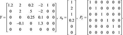
Let A and b of the general restricted linear Equation (1) be
(14)
The matrix Y is
Note that
, but
. If take
, then
. Here, we choose
in (4). Thus, it can be seen as the method given in [4] . The errors ,
,  , and
, and  of (4) with
  and
and  are presented in Table 1. Numerical results given in Table 1 show that
 , but
, but . Thus, the limit of
  is not the solution of (1) presented by Proposition 2.
Theorem 6 Under the same conditions as in Theorem 5. The iterative scheme (4) is stable for solving (1), where .
.
Proof. Let  and
and  be numerical perturbations of
  and
and  given in (4), respectively. Thus, we can express as
 ,
, . If
. If  ,
,  , then
 ,
, . Here, we formally neglect quadratic terms containing
 ,
, . Since
 , we get

By (4), we derive
 (15)
(15)
From (9) and (4), we have  and
and

Table 1. Error results of (4) with ,
, .
.

Therefore, we obtain
 (16)
(16)
By (4), we have . Similarly, we have
 (17)
(17)
By (17) and (16), we derive
 (18)
(18)
Thus, by , we have
 (19)
(19)
If , then
  and for any k,

where . It follows that the iterative method (4) is asymptotically stable. □
4. Numerical Examples
In the section, we give an example to test the accuracy of our scheme (4), which is implemented by our main code given in Appendix, and make a comparison with the method given in [4] . We also apply our scheme to solve the restricted linear system (1) with taking different t and intial value.
Example 1 Consider the restricted linear system (1) with a coefficient matrix being random  of order
 , where
 , 900, 1000, 2000 of index one and random vectors
 . Let
. Let  be a random matrix. Take
 ,
,  , and a random vector
 . Here, we make a comparison the mean CPU time(MCT) and error bounds of our scheme (4) with those given by the method of [4] . The stopping criteria used is given as in [4] by

Numerical results given in Table 2 and Figure 1 show that the accuracy of our method is similar to those given in [4] and our method cost less time (MCT) than the method of [4] . We can see that, to obtain the similar accuracy, the MCT of our scheme is similar to those given in [4] from Figure 2.
Table 2. The mean CPU time (MCT) and error in Example 1.
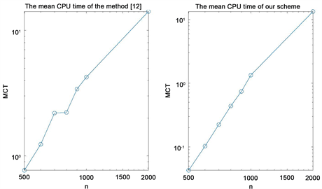
Figure 1. Error in example 1.
Example 2 Consider the general restricted linear Equation (1), where A and b is given as in (14). Here, we use the scheme (4) to solve the example. Let ,
, . Take
Obviously,  ,
,  ,
,  ,
,  , and
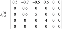
, and . To verify the accuracy of our method, we present the generalized inverse
  as
as
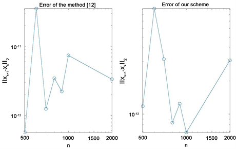
Figure 2. The MCT in Example 1.
Table 3. Error for (4) in Example 2 with .
.
To ensure , we take parameter
  in Table 3 and
  in Table 4, respectively. We present the errors
  ,
,  , and
, and  in 2-norm as
  in Table 3 and
  in Table 4, respectively.
Table 4. Error for (4) in Example 2 with .
.
From the numerical results given in Table 3 and Table 4, we can see that the scheme (4) has high order accuracy and these results given with  are better than those obtained by
 , respectively.
5. Conclusion
The high order iterative method has been derived for solving the general restricted linear equation. The convergence and stability of our method also have derived. Numerical experiments have presented to demonstrate the efficiency and accuracy.
Acknowledgements
This work was supported by the National Natural Science Foundation of China (No. 11061005, 11701119, 11761024), the Natural Science Foundation of Guangxi (No. 2017GXNSFBA198053), the Ministry of Education Science and Technology Key Project (210164), and the open fund of Guangxi Key laboratory of hybrid computation and IC design analysis (HCIC201607).
Cite this paper
Liu, X.J., Du, W.R., Yu, Y.M. and Qin, Y.H. (2018) Efficient Iterative Method for Solving the General Restricted Linear Equation. Journal of Applied Mathematics and Physics, 6, 418-428. https://doi.org/10.4236/jamp.2018.62039
References
- 1. Ben-Israel, A. and Greville, T.N.E. (2003) Generalized Inverses. Volume 15 of CMS Books in Mathematics/Ouvrages de Mathématiques de la SMC, 2nd Edition, Springer-Verlag, New York.
- 2. Chen, Y.L. (1993) A Cramer Rule for Solution of the General Restricted Linear Equation. Linear and Multilinear Algebra, 34, 177-186. https://doi.org/10.1080/03081089308818219
- 3. Wei, Y.M. and Wu, H.B. (2001) Splitting Methods for Computing the Generalized Inverse and Rectangular Systems. International Journal of Computer Mathematics, 77, 401-424. https://doi.org/10.1080/00207160108805075
- 4. Srivastava, S. and Gupta, D.K. (2015) An Iterative Method for Solving General Restricted Linear Equations. Applied Mathematics and Computation, 262, 344-353. https://doi.org/10.1016/j.amc.2015.04.047
- 5. Song, G.J., Wang, Q.-W. and Chang, H.-X. (2011) Cramer Rule for the Unique Solution of Restricted Matrix Equations over the Quaternion Skew field. Computers & Mathematics with Applications, 61, 1576-1589. https://doi.org/10.1016/j.camwa.2011.01.026
- 6. Chen, Y.L. (1997) Iterative Methods for Solving Restricted Linear Equations. Applied Mathematics and Computation, 86, 171-184. https://doi.org/10.1016/S0096-3003(96)00180-4
- 7. Wei, Y.M., Li, X.Z. and Wu, H.B. (2003) Subproper and Regular Splittings for Restricted Rectangular Linear System. Applied Mathematics and Computation, 136, 535-547. https://doi.org/10.1016/S0096-3003(02)00078-4
- 8. Yu, Y.M. (2008) PCR Algorithm for Parallel Computing the Solution of the General Restricted Linear Equations. Journal of Applied Mathematics and Computing, 27, 125-136. https://doi.org/10.1007/s12190-008-0062-3
- 9. Song, G.-J. and Dong, C.-Z. (2017) New Results on Condensed Cramer’s Rule for the General Solution to Some Restricted Quaternion Matrix Equations. Journal of Applied Mathematics and Computing, 53, 321-341. https://doi.org/10.1007/s12190-015-0970-y
- 10. Cai, J. and Chen, G.L. (2007) On Determinantal Representation for the Generalized Inverse and Its Applications. Numerical Linear Algebra with Applications, 14, 169-182. https://doi.org/10.1002/nla.513
- 11. Liu, X.J., Zhu, G.Y., Zhou, G.P. and Yu, Y.M. (2012) An Analog of the Adjugate Matrix for the Outer Inverse . Mathematical Problems in Engineering, Article ID: 591256.
- 12. Roger, A.H. and Johnson, C.R. (2013) Matrix Analysis. 2nd Edition, Cambridge University Press, Cambridge.
- 13. Liu, X.J., Jin, H.W. and Yu, Y.M. (2013) Higher-Order Convergent Iterative Method for Computing the Generalized Inverse and Its Application to Toeplitz Matrices. Linear Algebra and Its Applications, 439, 1635-1650. https://doi.org/10.1016/j.laa.2013.05.005
- 14. Srivastava, S., Stanimirovic, P.S., Katsikis, V.N. and Gupta, D.K. (2017) A Family of Iterative Methods with Accelerated Convergence for Restricted Linear System of Equations. Mediterranean Journal of Mathematics, 14, 222. https://doi.org/10.1007/s00009-017-1020-9
Appendix
function hocigrlscm( )
)
 ;
; ;
;
fprintf('


 )
)
fprintf('------------------------BEGING---------------------------- )
)
 ;
; ;
; 
for ,
,
tic; ;
; ;
; ;
;
for 
 ;
;
 ; % compute
end
 ;
;
 ;
; 
clear ;
;


 itm = toc;
if ,
, ; break, end
end % END it