Modern Mechanical Engineering, 2011, 1, 25-30
doi:10.4236/mme.2011.12004 Published Online November 2011 (http://www.SciRP.org/journal/mme)
Modeling of Piezoelectric Actuators Based on a New
Rate-Independent Hysteresis Model
Jingyang Peng, Xiongbiao Chen
Department of Mechanical Engineering, University of Saskatchewan, Saskatoon, Canada
Received September 27, 2011; revised October 28, 2011; accepted November 5, 2011
Abstract
Accurate model representatives of piezoelectric actuators (PEAs) are important for both understanding the
dynamic behaviors of PEAs and control scheme development. However, among the existing models, the
most widely used classical Preisach hysteresis model are incapable of representing the commonly-encoun-
tered one-sided (non-negative voltage input range) hysteresis behaviors of PEAs. To solve this problem, a
new rate-independent hysteresis model was developed for the one-sided hysteresis and then integrated with
the models representative of creep and dynamics to form a single model for the PEAs. Experiments were
carried out to validate the developed models.
Keywords: Piezoelectric Actuator, Hysteresis
1. Introduction
Piezoelectric actuators (PEAs) have been widely used in
micro-/nano-positioning systems due to their fine displace-
ment resolution and large actuation force [1]. In such
applications, accurate models of PEAs are usually requi-
red for both understanding of their dynamic behaviors
and controller design. A widely-used category of PEA mo-
dels takes the form of a cascade of three sub-models, each
of which representing the effect of hysteresis, creep, and
vibration dynamics, respectively, e.g. [2]. While the mod-
eling of the vibration dynamics and creep has been well
addressed in the literature, there are still problems with the
modeling of hysteresis. Most commercially available PEAs
have a non-negative input voltage range and their corre-
sponding hysteresis behaviors subject to such one-sided
input range are referred to as one-sided hysteresis, as shown
in Figure 1, which contains an initial ascending curve in
addition to the hysteresis loops. It is observed in the au-
thors’ earlier study [3] that the classical Preisach (CP) hys-
teresis model [4] cannot represent such one-sided hys-
teresis since it can not represent the initial ascending
curve. This deficiency of the CP hysteresis model has
been neglected in the literature, e.g. [5-8]. This problem
of modeling the one-sided hysteresis was solved in [3] by
developing a new rate-independent (RI) hysteresis model
based on a novel hysteresis operator.
On this basis, in this paper, this new RI hysteresis model
Figure 1. One-sided hysteresis behavior measured from a
PEA subjected to non-negative voltage input.
is integrated with a vibration sub-model and a creep sub-
model to form an integrated model for PEAs. The pa-
rameter estimation scheme for such a model of PEAs is
also developed. Experiments were conducted and the re-
sults obtained were compared with simulation results to
validate the model developed.
2. Outline of the Rate-Independent (RI)
Hysteresis Model
The RI hysteresis model developed in [3] represents one-
sided hysteresis behaviors as the combined effects of an
infinite number of hysteresis operators, one of which is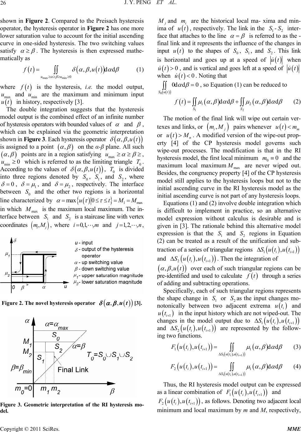

J. Y. PENG ET AL.
26
shown in Figure 2. Compared to the Preisach hysteresis
operator, the hysteresis operator in Figure 2 has one more
lower saturation value to account for the initial ascending
curve in one-sided hysteresis. The two switching values
satisfy

 . The hysteresis is then expressed mathe-
matically as
 


maxmin 0
,, dd
uu
ft ut


 
 
 (1)
where

f
t is the hysteresis, i.e. the model output,
and min
u are the maximum and minimum input
in history, respectively [3].
max
u

ut
The double integration suggests that the hysteresis
model output is the combined effect of an infinite number
of hysteresis operators with bounded values of

and

,
which can be explained via the geometric interpretation
shown in Figure 3. Each hysteresis operator


ut

,, 



is assigned to a point

,

 on the α-β plane. All such

,


 points are in a region satisfying max u

 
T
 ,
min which is referred to as the limiting triangle 0.
According to the values of
0u



,,ut 
S S
, 0 is divided
into three regions denoted by 0, 1, and 2, where
T
S
0

, 1

 , and 2

 , respectively. The interface
between and the other two regions is a horizontal
0
S
line characterized by



1max
max 0utMM  

in which max is the maximum local maximum. The in-
terface between and is a staircase line with vertex
M

1
S2 S
coordinates , where ,
ij
mM 0,1, ,im

 and 1, 2,,jn

,
Figure 2. The novel hysteresis operator

 
,,  ut [3].
Figure 3. Geometric interpretation of the RI hysteresis mo-
del.
j
M
and are the historical local ma- xima and min-
ima of
i
m


ut , respectively. The link in the 1-2 inter-
face that attaches to the line
S S

  is referred to as the -
final link and it represents the influence of the changes in
input


ut to the shapes of , , and . This link
0
S S1 2 S
is horizontal and goes up at a speed of


ut
 when


0ut 
, and is vertical and goes left at a speed of


ut

when


0ut


0d
. Noting that
 
0
Sut
d 0 

 , so Equation (1) can be reduced to




12
12
,dd ,dd
SS
ft

  
 (2)
The motion of the final link will wipe out certain ver-
texes and links, or


,
ij
mM pairs whenever


m
ut m
or


n
ut M. A modified version of the wipe-out prop-
erty [4] of the CP hysteresis model governs such
wipe-out processes. The modification is that in the RI
hysteresis model, the first local minimum 0 and the
maximum local maximummax are never wiped out.
Besides, the congruency property [4] of the CP hysteresis
model still applies to the hysteresis loops but not to the
initial ascending curve in the RI hysteresis model as the
initial ascending curve is not part of any hysteresis loops.
0m
M
Equations (1) and (2) involve double integration which
is difficult to implement in practice, so an alternative
model expression without calculus is desirable and is
given in [3]. The rationale behind this alternative model
expression is that the 1 and 2 regions in Equation
(2) can be treated as a result of the unification and sub-
S S
traction of a series of triangular regions



 
11
,
ii
Sut ut


and






2
,
ii
Sut ut

1 . Then the integration of




,,ut  over each of such triangular regions can be
pre-identified and used to calculate

f
t through a series
of adding and subtracting operations.
Specifically, each of such triangular regions represents
the shape change in 1 or 2as the input changes mo-
notonically between two adjacent extrema
S S


i
ut and


1i
ut
 in the input history which are not wiped-out. The
changes in the model output due to





11
Su t

,
ii
t u
and






2 are represented by the follow-
ing two functions.
1
,
i
Sut ut
i








  
11
11 1
,
,,
ii
ii
Sut ut
Fut utdd








 (3)







 

11
21 1
,
,,
ii
ii
Sut ut
Fut utdd

 



 (4)
Thus, the RI hysteresis model output can be expressed
as a linear combination of
 


11
,
ii
Fut ut
 and






2
,
ii
Fut ut
1
, as follows. Denoting two adjacent local
minimum and local maximum by m and M, respectively,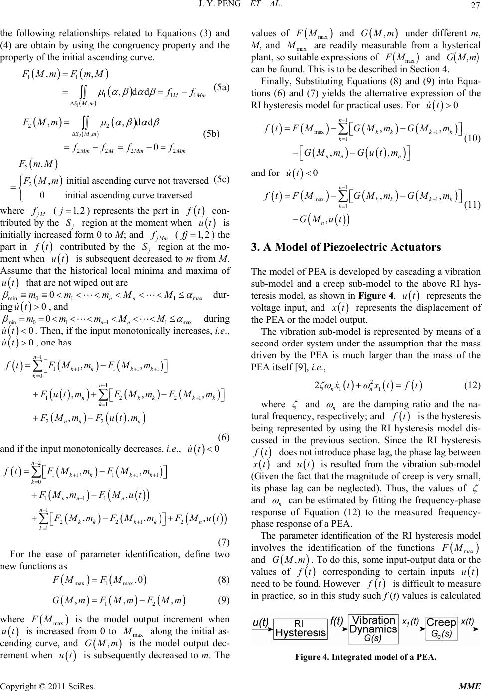

J. Y. PENG ET AL. 27
1
the following relationships related to Equations (3) and
(4) are obtain by using the congruency property and the
property of the initial ascending curve.



1
11
11
,
,,
,dd
M
Mm
SMm
FMm FmM
f
f  



 
(5a)
 

2
22
,
2222
,,dd
0
SMm
M
m MMmMm
FMm
f
fff






(5b)


2
2, initial ascending curve not traversed
0 initial ascending curve traversed
FMm 


,FmM
(5c)
where
j
M
f
() represents the part in 1, 2j


f
t con-
tributed by the
j
S region at the moment when


ut is
initially increased form 0 to M; and
j
Mm
f
(1, 2fj

) the
part in


f
t contributed by the
j
S
M
region at the mo-
ment when is subsequent decreased to m from M.
Assume that the historical local minima and maxima of
that are not wiped out are
mi

ut
1
mm

ut
n 01nn
mmax M0

 

0
00

mm

mM M
  dur-
ing , and
111 maxnn
ut

mi n

 
 during
. Then, if the input monotonically increases, i.e.,
, one has

0
0
1n
 

ut 


ut 

  
  
 

11 111
0
1
122
1
22
,,
,,
,,
kk kk
k
n
nkkk
k
nn n
ftFM mFM m
FutmF M mF Mm
FMm Futm
 




 

  





1
,
k
(6)
and if the input monotonically decreases, i.e.,


0ut



 



   
2
11 111
0
111
1
2212
1
,,
,,
,,
n
kk kk
k
nn n
n
kkk kn
k
ftFM mFM m
FM mFMut

,
F
MmFMmFMut
















(7)
For the ease of parameter identification, define two
new functions as

max1max ,0FMFM


,

(8)

12
,,GMmF MmFMm (9)
where is the model output increment when
is increased from 0 to max along the initial as-
cending curve, and is the model output dec-
rement when is subsequently decreased to m. The
values of

max
FM

ut

ut M

,GMm



max
FM
M
and under different m,
M, and max are readily measurable from a hysterical
plant, so suitable expressions of and

,GMm
FM


max


,GMm
0

k
m
can be found. This is to be described in Section 4.
Finally, Substituting Equations (8) and (9) into Equa-
tions (6) and (7) yields the alternative expression of the
RI hysteresis model for practical uses. For

ut

 

1
1
1
,,
n
k
k
nn
ft M
m




max
FM
GM


,,
kk
GMm
Gut m


n
G


 





(10)
and for


0ut




 
1
1
1
,,
n
k
k
ft M
t




max
,
n
FM
GM u

kk
GMm

G

k
m

  



(11)
3. A Model of Piezoelectric Actuators
The model of PEA is developed by cascading a vibration
sub-model and a creep sub-model to the above RI hys-
teresis model, as shown in Figure 4.


ut represents the
voltage input, and


x
t represents the displacement of
the PEA or the model output.
The vibration sub-model is represented by means of a
second order system under the assumption that the mass
driven by the PEA is much larger than the mass of the
PEA itself [9], i.e.,


2
11nn

2
x
txt  ft 
 (12)
where

and n

are the damping ratio and the na-
tural frequency, respectively; and


f
t is the hysteresis
being represented by using the RI hysteresis model dis-
cussed in the previous section. Since the RI hysteresis


f
t does not introduce phase lag, the phase lag between


x
t and


ut is resulted from the vibration sub-model
(Given the fact that the magnitude of creep is very small,
its phase lag can be neglected). Thus, the values of

and n

can be estimated by fitting the frequency-phase
response of Equation (12) to the measured frequency-
phase response of a PEA.
The parameter identification of the RI hysteresis model
involves the identification of the functions


max
FM
and


,mGM. To do this, some input-output data or the
values of


f
t corresponding to certain inputs


ut
need to be found. However


f
t is difficult to measure
in practice, so in this study such f (t) values is calculated
Figure 4. Integrated model of a PEA.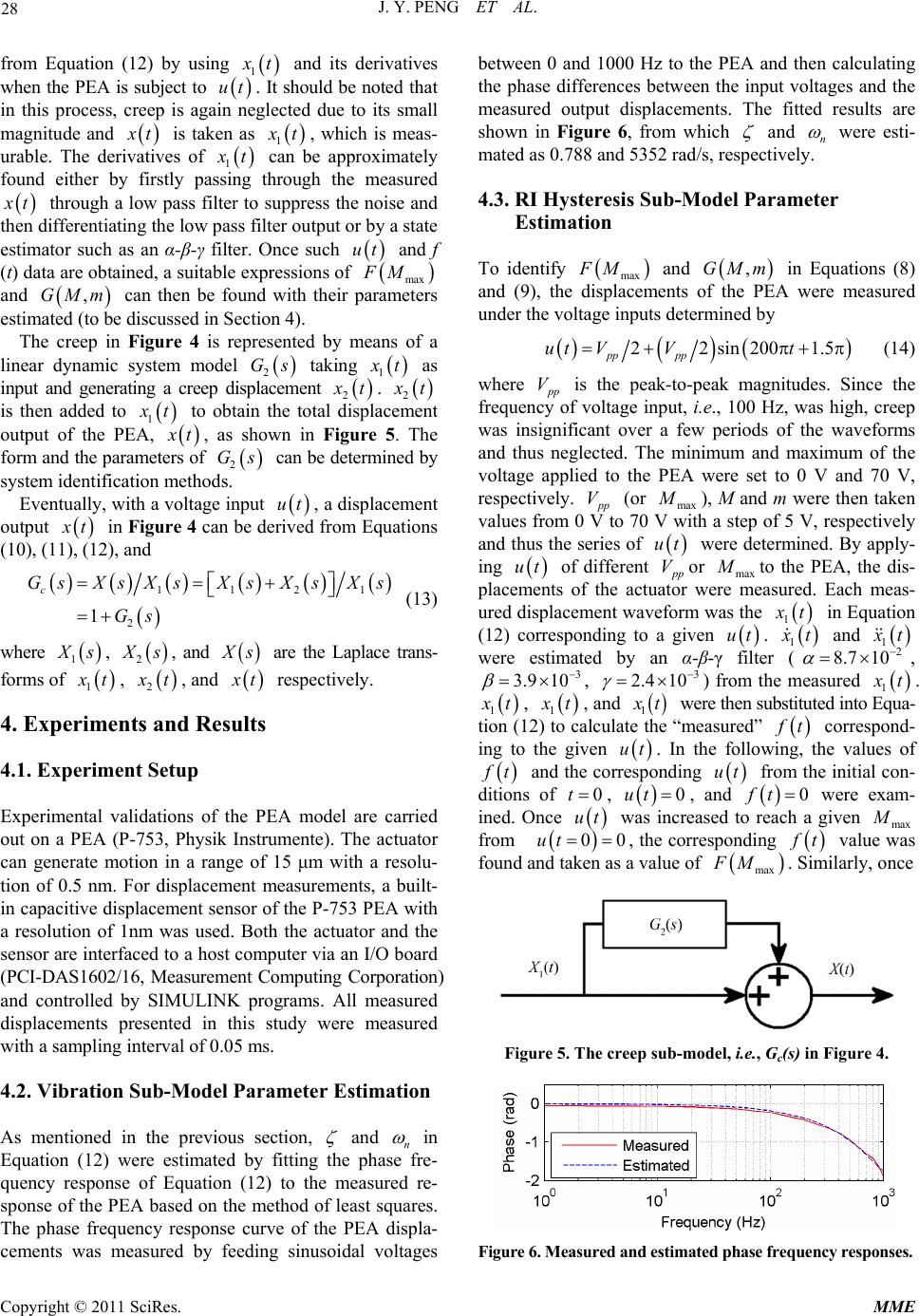

J. Y. PENG ET AL.
28
from Equation (12) by using

1
x
t and its derivatives
when the PEA is subject to


ut . It should be noted that
in this process, creep is again neglected due to its small
magnitude and

x
t is taken as

1
x
t, which is meas-
urable. The derivatives of


1
x
t can be approximately
found either by firstly passing through the measured

x
t through a low pass filter to suppress the noise and
then differentiating the low pass filter output or by a state
estimator such as an α-β-γ filter. Once such


ut and f
(t) data are obtained, a suitable expressions of


max
FM
and can then be found with their parameters
estimated (to be discussed in Section 4).

,GMm

The creep in Figure 4 is represented by means of a
linear dynamic system model taking

2
Gs


1
x
t

as
input and generating a creep displacement 2

x
t.


2
x
t
is then added to

1
x
t

to obtain the total displacement
output of the PEA,

x
t, as shown in Figure 5. The
form and the parameters of


s
2 can be determined by
system identification methods.
G
Eventually, with a voltage input , a displacement
output

ut

x
t in Figure 4 can be derived from Equations
(10), (11), (12), and
 





1121
2
1
c
GsXsXsXsX sXs
Gs


 (13)
where


1
X
s,

2
X
s, and


X
s are the Laplace trans-
forms of

1
x
t,

2
x
t, and

x
t respectively.
4. Experiments and Results
4.1. Experiment Setup
Experimental validations of the PEA model are carried
out on a PEA (P-753, Physik Instrumente). The actuator
can generate motion in a range of 15 μm with a resolu-
tion of 0.5 nm. For displacement measurements, a built-
in capacitive displacement sensor of the P-753 PEA with
a resolution of 1nm was used. Both the actuator and the
sensor are interfaced to a host computer via an I/O board
(PCI-DAS1602/16, Measurement Computing Corporation)
and controlled by SIMULINK programs. All measured
displacements presented in this study were measured
with a sampling interval of 0.05 ms.
4.2. Vibration Sub-Model Parameter Estimation
As mentioned in the previous section,

and n

in
Equation (12) were estimated by fitting the phase fre-
quency response of Equation (12) to the measured re-
sponse of the PEA based on the method of least squares.
The phase frequency response curve of the PEA displa-
cements was measured by feeding sinusoidal voltages
between 0 and 1000 Hz to the PEA and then calculating
the phase differences between the input voltages and the
measured output displacements. The fitted results are
shown in Figure 6, from which

and n

were esti-
mated as 0.788 and 5352 rad/s, respectively.
4.3. RI Hysteresis Sub-Model Parameter
Estimation
To identify


max
FM and


,GM in Equations (8)
and (9), the displacements of the PEA were measured
under the voltage inputs determined by
m





22 sin2001.5
pp pp
ut VVt


(14)
where
p
p is the peak-to-peak magnitudes. Since the
frequency of voltage input, i.e., 100 Hz, was high, creep
was insignificant over a few periods of the waveforms
and thus neglected. The minimum and maximum of the
voltage applied to the PEA were set to 0 V and 70 V,
respectively.
V
p
p (or max ), M and m were then taken
values from 0 V to 70 V with a step of 5 V, respectively
and thus the series of
VM


ut were determined. By apply-
ing


ut of different
p
p
Vor max to the PEA, the dis-
placements of the actuator were measured. Each meas-
ured displacement waveform was the
M

1
x
t

in Equation
(12) corresponding to a given . 1

ut
x
t
 and


1
x
t

2
10 were estimated by an α-β-γ filter (8.7 

 ,
3
 3.9 10

 , 3 102.4 

 ) from the measured


1
x
t.


1
x
t,


1
x
t, and


1
x
t were then substituted into Equa-
tion (12) to calculate the “measured”

f
t correspond-
ing to the given


ut . In the following, the values of


f
t and the corresponding from the initial con-
ditions of t

ut

0

,


0ut

, and were exam-
ined. Once

ft0


ut was increased to reach a given max
from
M


00ut

, the corresponding

f
t

value was
found and taken as a value of . Similarly, once

ma
FM x
Figure 5. The creep sub-model, i.e., Gc(s) in Figure 4.
Figure 6. Measured and estimated phase frequency responses.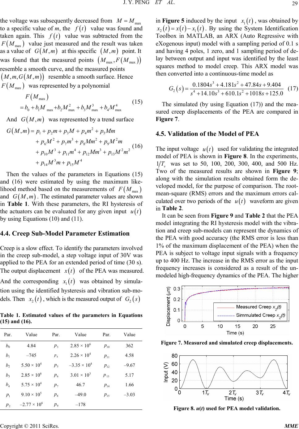

29 J. Y. PENG ET AL.
the voltage was subsequently decreased from max MM

to a specific value of m, the

f
t value was found and
taken again. This


f
t

,m
value was subtracted from the
value just measured and the result was taken
as a value of at this specific


max
FM

GM

,
M
m point. It
was found that the measured points

 
MFM



max max
,
resemble a smooth curve, and the measured points


,, ,
M
mG M m

FM
resemble a smooth surface. Hence
max was represented by a polynomial

max
23
01max2 max3 max4max
FM
bbMbMbMbM 4

2
(15)
And was represented by a trend surface

,GMm

2
12 345
232 2
678 9
343 2
1011 1213
34
14 15
,GM mppmpMpmpMm
pMpmpMmpM m
pMpmpMm pMm
pMm pM
 
 
 

(16)
Then the values of the parameters in Equations (15)
and (16) were estimated by using the maximum like-
lihood method based on the measurements of


max
FM
and


,GMm. The estimated parameter values are shown
in Table 1. With these parameters, the RI hysteresis of
the actuators can be evaluated for any given input


ut
by using Equations (10) and (11).
4.4. Creep Sub-Model Parameter Estimation
Creep is a slow effect. To identify the parameters involved
in the creep sub-model, a step voltage input of 30V was
applied to the PEA for an extended period of time (30 s).
The output displacement

x
t of the PEA was measured.
And the corresponding


1
x
t was obtained by simula-
tion using the identified hysteresis and vibration sub-mo-
dels. Then


2
x
t, which is the measured output of


2
Gs
Table 1. Estimated values of the parameters in Equations
(15) and (16).
Par. Value Par. Value Par. Value
b0 4.84 3
p 2.85 × 106 10 p 362
b1 –745 4
p2.26 × 104 11
p 4.58
b2 5.50 × 104 5
p –3.35 × 104 12 p –9.67
b3 2.85 × 106 6
p 3.01 × 103 13 p 5.17
4
b 5.75 × 104 7
p 46.7 14
p 1.66
1
p 9.10 × 105 8
p –49.0 15 p –3.03
2
p –2.77 × 106 9
p –178
in Figure 5 induced by the input

1
x
t, was obtained by






21
x
txtxt . By using the System Identification
Toolbox in MATLAB, an ARX (Auto Regressive with
eXogenous input) model with a sampling period of 0.1 s
and having 4 poles, 1 zero, and 1 sampling period of de-
lay between output and input was identified by the least
squares method to model creep. This ARX model was
then converted into a continuous-time model as

32
2432
0.18044.18147.849.404
14.10610.11018 125.0
sss
Gs
s
sss

 (17)
The simulated (by using Equation (17)) and the mea-
sured creep displacements of the PEA are compared in
Figure 7.
4.5. Validation of the Model of PEA
The input voltage


ut used for validating the integrated
model of PEA is shown in Figure 8. In the experiments,
1v T was set to 50, 100, 200, 300, 400, and 500 Hz.
Two of the measured results are shown in Figure 9;
along with the simulation results obtained form the de-
veloped model, for the purpose of comparison. The root-
mean-square (RMS) errors and the maximum errors cal-
culated over two periods of the waveform are given
in Table 2.

ut
It can be seen from Figure 9 and Tabl e 2 that the PEA
model integrating the RI hysteresis model with the vibra-
tion and creep sub-models can represent the dynamics of
the PEA with good accuracy (the RMS error is less than
1% of the maximum displacement of the PEA) when the
PEA is subject to voltage input signals with a frequency
up to 400 Hz. The increase in the RMS error as the input
frequency increases is considered as a result of the un-
modeled high-frequency dynamics of the PEA. The higher
Figure 7. Measured and simulated creep displacements.
Figure 8. u(t) used for PEA model validation.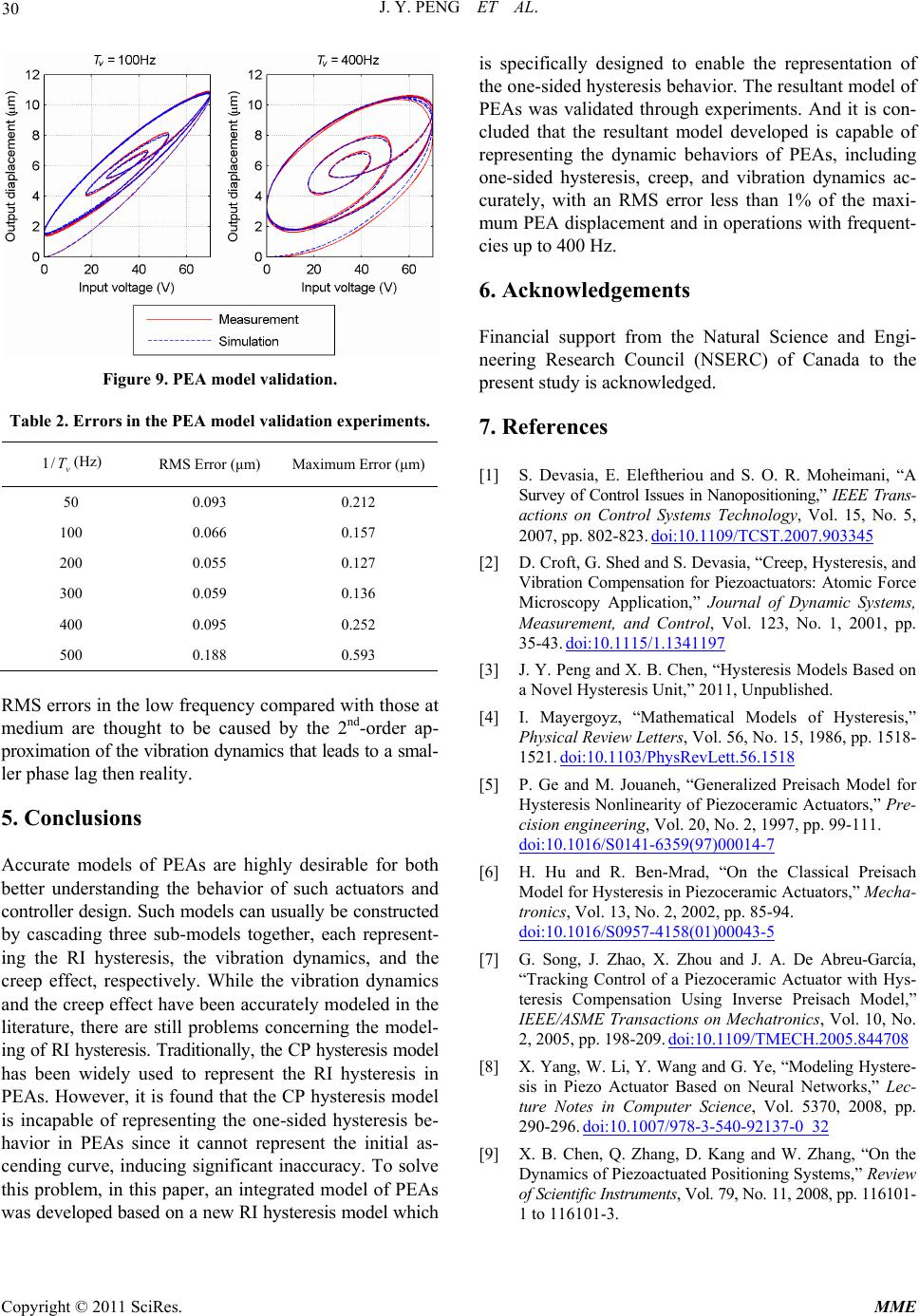

J. Y. PENG ET AL.
30
is specifically designed to enable the representation of
the one-sided hysteresis behavior. The resultant model of
PEAs was validated through experiments. And it is con-
cluded that the resultant model developed is capable of
representing the dynamic behaviors of PEAs, including
one-sided hysteresis, creep, and vibration dynamics ac-
curately, with an RMS error less than 1% of the maxi-
mum PEA displacement and in operations with frequent-
cies up to 400 Hz.
6. Acknowledgements
Financial support from the Natural Science and Engi-
neering Research Council (NSERC) of Canada to the
present study is acknowledged.
Figure 9. PEA model validation.
Table 2. Errors in the PEA model validation experiments. 7. References
v
T/1 (Hz) RMS Error (μm) Maximum Error (μm)
50 0.093 0.212
100 0.066 0.157
200 0.055 0.127
300 0.059 0.136
400 0.095 0.252
500 0.188 0.593
[1] S. Devasia, E. Eleftheriou and S. O. R. Moheimani, “A
Survey of Control Issues in Nanopositioning,” IEEE Trans-
actions on Control Systems Technology, Vol. 15, No. 5,
2007, pp. 802-823. doi:10.1109/TCST.2007.903345
[2] D. Croft, G. Shed and S. Devasia, “Creep, Hysteresis, and
Vibration Compensation for Piezoactuators: Atomic Force
Microscopy Application,” Journal of Dynamic Systems,
Measurement, and Control, Vol. 123, No. 1, 2001, pp.
35-43. doi:10.1115/1.1341197
[3] J. Y. Peng and X. B. Chen, “Hysteresis Models Based on
a Novel Hysteresis Unit,” 2011, Unpublished.
RMS errors in the low frequency compared with those at
medium are thought to be caused by the 2nd-order ap-
proximation of the vibration dynamics that leads to a smal-
ler phase lag then reality.
[4] I. Mayergoyz, “Mathematical Models of Hysteresis,”
Physical Review Letters, Vol. 56, No. 15, 1986, pp. 1518-
1521. doi:10.1103/PhysRevLett.56.1518
[5] P. Ge and M. Jouaneh, “Generalized Preisach Model for
Hysteresis Nonlinearity of Piezoceramic Actuators,” Pre-
cision engineering, Vol. 20, No. 2, 1997, pp. 99-111.
doi:10.1016/S0141-6359(97)00014-7
5. Conclusions
Accurate models of PEAs are highly desirable for both
better understanding the behavior of such actuators and
controller design. Such models can usually be constructed
by cascading three sub-models together, each represent-
ing the RI hysteresis, the vibration dynamics, and the
creep effect, respectively. While the vibration dynamics
and the creep effect have been accurately modeled in the
literature, there are still problems concerning the model-
ing of RI hysteresis. Traditionally, the CP hysteresis model
has been widely used to represent the RI hysteresis in
PEAs. However, it is found that the CP hysteresis model
is incapable of representing the one-sided hysteresis be-
havior in PEAs since it cannot represent the initial as-
cending curve, inducing significant inaccuracy. To solve
this problem, in this paper, an integrated model of PEAs
as developed based on a new RI hysteresis model which
[6] H. Hu and R. Ben-Mrad, “On the Classical Preisach
Model for Hysteresis in Piezoceramic Actuators,” Mecha-
tronics, Vol. 13, No. 2, 2002, pp. 85-94.
doi:10.1016/S0957-4158(01)00043-5
[7] G. Song, J. Zhao, X. Zhou and J. A. De Abreu-García,
“Tracking Control of a Piezoceramic Actuator with Hys-
teresis Compensation Using Inverse Preisach Model,”
IEEE/ASME Transactions on Mechatronics, Vol. 10, No.
2, 2005, pp. 198-209. doi:10.1109/TMECH.2005.844708
[8] X. Yang, W. Li, Y. Wang and G. Ye, “Modeling Hystere-
sis in Piezo Actuator Based on Neural Networks,” Lec-
ture Notes in Computer Science, Vol. 5370, 2008, pp.
290-296. doi:10.1007/978-3-540-92137-0_32
[9] X. B. Chen, Q. Zhang, D. Kang and W. Zhang, “On the
Dynamics of Piezoactuated Positioning Systems,” Review
of Scientific Instruments, Vol. 79, No. 11, 2008, pp. 116101-
1 to 116101-3.
w
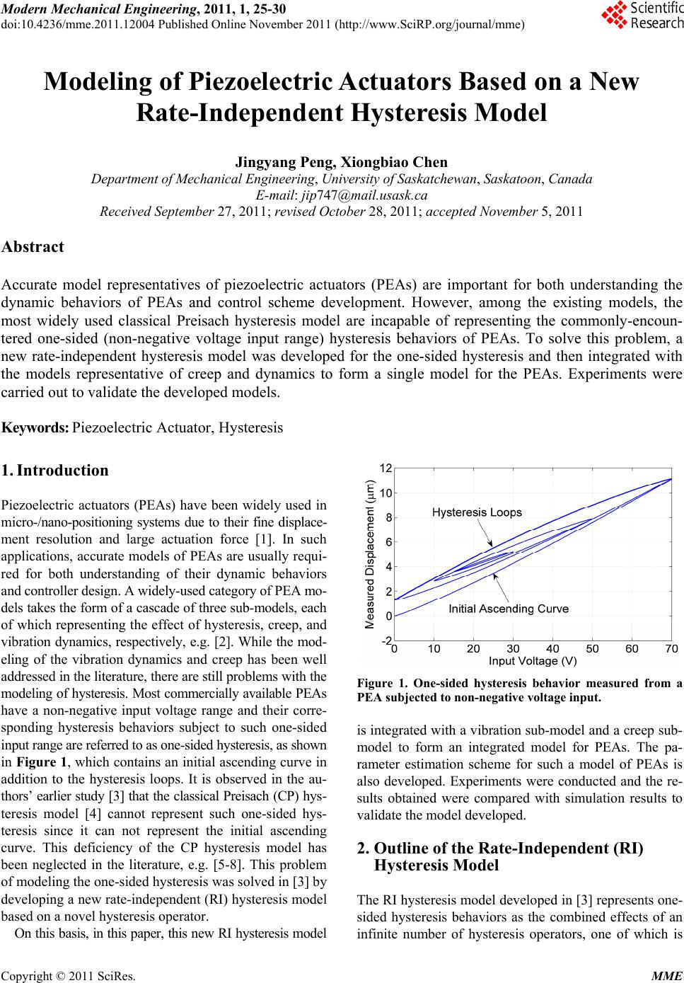