ABSTRACT

A weather-adaptive forward collision warning (FCW) system was presented by applying local features for vehicle detection and global features for vehicle verification. In the system, horizontal and vertical edge maps are separately calculated. Then edge maps are threshold by an adaptive threshold value to adapt the brightness variation. Third, the edge points are linked to generate possible objects. Fourth, the objects are judged based on edge response, location, and symmetry to generate vehicle candidates. At last, a method based on the principal component analysis (PCA) is proposed to verify the vehicle candidates. The proposed FCW system has the following properties: 1) the edge extraction is adaptive to various lighting condition; 2) the local features are mutually processed to improve the reliability of vehicle detection; 3) the hierarchical schemes of vehicle detection enhance the adaptability to various weather conditions; 4) the PCA-based verification can strictly eli- minate the candidate regions without vehicle appearance.

Keywords:

Forward Collision Warning (FCW), Advanced Driver Assistance System (ADAS), Weather Adaptive, Principal Component Analysis (PCA)

1. Introduction

To avoid the traffic accidents and to decrease injuries and fatalities, many advanced driving assistance systems (ADASs) have been developed paying more regard to situations on road for drivers, such as forward collision warning (FCW), lane departure warning (LDW), blind spot detection (BSD), etc. Based on our previous studies [1] [2] [3], this study focuses on developing a FCW system.

Extensive studies have been proposed for vision-based FCW systems [4] [5] [6] [7]. Sun et al. [4] and Sivaraman et al. [5] generally divided the vision-based vehicle detection methods into three categories: knowledge-based, motion- based, and stereo-based methods. Knowledge-based methods integrate many features of vehicles to recognize preceding vehicles in images. Most of these methods are implemented by two steps: hypothesis generation (HG) and hypothesis verification (HV) [4]. The HG step detects all possible vehicle candidates in an image; the vehicle candidates are then confirmed by the HV step to ensure correct detections.

Due to the rigidness and the specific appearance of vehicles, many features such as edges, shadow, symmetry, texture, color, and intensity can be observed in images. The features used in knowledge-based methods can be further divided into global features and local features according to whether the vehicle appearance is considered when using the features. A usable FCW system should be stable in various weather conditions and in various background scenes. Furthermore, the system should get high detecting rate with fewer false alarms by utilizing both local- and global features.

The weather adaptability of edge information is much better than other local features such as shadow and symmetry. The contour of a vehicle can represent by horizontal and vertical edges. However, the local edge features are not strict enough to describe vehicle appearance. The appearance based verification is better and need to support the vehicle detection based on edge information.

We here propose a FCW system combining the advantage of the global features and local features to improve the reliability of vehicle detection. The local feature is invariant to vehicle direction, lighting condition, and partial occlusion. The global feature is used to search objects in the image base on whole vehicle configuration. In the detection stage, all vehicle candidates are located according to the local as many as possible to avoid missing targets; in the verification stage, each candidate is confirmed as real target by the global as strictly as possible to reduce the false alarms.

The proposed FCW system detects vehicles relying on edges; thereby the proposed system can work well under various weather conditions. At first, the lane detector [1] [2] is performed to limit the searching region of preceding vehicles. Then an adaptive threshold is used to obtain bi-level horizontal and vertical edges in the region. The vehicle candidate is generated depending on a valid horizontal edge and the geometry constrains vertical edges at two ends of the horizontal edge. In verification stage, the vehicle candidates are verified by vehicle appearance and principal component analysis (PCA). A principal component set is obtained by applying PCA to a set of canonical vehicle images. These components are used to dominate the appearance of vehicle-like regions; therefore, the regions of vehicle-like objects can be well reconstructed by the principal components. The closer the distance between an image and its reconstruction image is, the higher the probability of the object on the image being a vehicle is.

2. Vehicle Detection

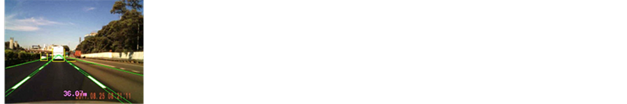
Edge information is an important feature for detecting vehicles in an image, especially the horizontal edges of underneath shadows. In the detection stage, vehicle candidates are generated based on local edge features. Firstly, the appropriate edge points are extracted in the region of interest (ROI) defined by lane marks as shown in Figure 1. Then, the significant horizontal edges indicating vehicle locations are refined. The negative horizontal edges (NHE) are thought belonging to underneath shadow. The positive horizontal edges (PHE) are mostly formed by bumper, windshield and roof of vehicles. For each kind of horizontal edges with different property, a specific procedure to find vertical borders of vehicles is applied around each horizontal edge. Finally, the horizontal edges and vertical borders are used to find the bounding boxes of vehicle candidates.

The horizontal edges are expected belonging to underneath shadows or vehicle body. Considering the sunlight influences, the horizontal edges belonging to underneath shadows are further divided into the moderate or the long by edge widths. The procedures for searching the paired vertical borders are designed according to the specific properties of different kinds of horizontal edges. In the proposed vehicle detection, three detecting methods (Case-1, Case-2, and Case- 3) are respectively designed to generate vehicle candidates based on the horizontal edges of underneath shadows, long underneath shadows, and vehicle bodies. In the situations of clear weather with less influence from sunlight, the underneath shadows are distinct and the widths of shadows are similar to vehicle width; Case-1 method proposed based on horizontal edges of moderate underneath shadows is adequately used to generate candidates. In the situations of sunny weather with lengthened shadow, there is the strong possibility that only one vertical border is searched by using Case-1 method; Case-2 method is proposed based on horizontal edge of long underneath shadows to search two corresponding vertical borders in a larger region, as shown in Figure 2. In the situations of bad weather disturbed by water spray and reflection, the underneath shadows are not reliable and are not observed at the worst; Case-3 method base on vehicle bodies is applied in a different way to retrieve the missing cases of using Case-1 and 2 methods.

If the only one vertical edge of the NHE is at the right side, it is taken as the

right boundary of the window. The left boundaries of all windows are respectively set at the x-positions which are 0.3 w_lane to 0.8 w_lane away from the right boundaries, and vice versa. The symmetry of the vertical edge points in the window is calculated by

, (1)

where h and w are the height and the width of the window, x_i and y_j are the x- and y-locations in the window, eng(x_i, y_j) is the energy of symmetry at (x_i, y_j) defined by

, (2)

where I_ep(x, y) is the value of the edge point map I_ep at (x, y) and I_ep is one of the vertical, the positive horizontal, and the negative horizontal edge point maps which are I_vep, I_{p_hep}, and I_{n_hep}.

The horizontal edges in Case-3 are the edges of the vehicle body, though the components which they belong to are unknown. The y-positions of the horizontal edges can’t indicate the y-positions of the candidate bottoms, which only gives a hint of the vehicle’s location. In the image, two vertical edges could be detected at vehicle sides, which are similar to each other in length and y-posi- tion. Therefore, two characteristic vertical edges are extracted from the areas around two endpoints of the horizontal edge, respectively. The distance and the y-position overlapping between two vertical edges are used to determine candidate bottom.

Firstly, the areas for searching the vertical edges are set extending upward and downward from the horizontal edge endpoints, as the gray regions in Figure 3.

According to the candidate bottoms, the images of the vehicle candidates are extracted with ratio height/width being 1. In the detecting result, the candidate locations are represented by “U” shape bounding boxes. The bottom of a “U” shape bounding box is the candidate bottom. The left and right margins of the

bounding box are defined as the vertical line segments from (x^l, y^l) to (x^l, y^l +) and from (x^r, y^(r)) to (x^r, y^r +), respectively. is the width of the candidate bottom, that is = x^r ? x^l. Each horizontal edge is individually determined if it belongs to a vehicle candidate. Around one vehicle target, there might be many bounding boxes which are set according to the horizontal edges at different y-positions. To delete the repetitions, the candidate being most closes to the host vehicle in a candidate group is reserved for the rest processes. That is, the bounding box with smallest y-position in image is reserved.

3. Vehicle Verification

In the verification stage, the vehicle candidates are determined applying PCA reconstruction. The reconstruction images are obtained according to the images of pre-trained eigenvehicles. Then, the image comparison methods are used to evaluate the likelihood of the vehicle candidates to e vehicle.

3.1. The Principle and Procedure of PCA-based Verification

Principal components analysis (PCA) is a statistical technique used to analyze and simplify a data set. Each principle component (eigenvector) is obtained with a corresponding data variance (eigenvalue). The larger the corresponding variance is, the more important the data information contained by the principle component is. For application of reducing data dimensionality, the principle components are sorted by the corresponding variance; and the original data are projected onto the principle components with the largest m variance. PCA is widely performed to image recognition and compression.

3.2. Eigenvehicle Generation

The images of the eigenvectors obtained by applying PCA to vehicle images are called “eigenvehicles”. To generate a set of eigenvehicles, a training set of preceding vehicle images cropped from on-road driving videos are prepared. The on-road driving videos are captured under various weather conditions; the training images are collected with various vehicle types, in various distance far from the own vehicle, and at the own/adjacent lane. The cropped images of preceding vehicles are firstly resized to 32 ´ 32. For each resized image, the edge map is produced and then normalized by letting the sum of edge values being equal to 1. The normalized edge maps as the training images are represented as vectors G₁, G₂, …,and G_M of size N, where M is the number of training images and N = 32 ´ 32.

Only the leading eigenvehicles are applied in the verification of vehicle candidates. The sixteen leading eigenvehicles with largest eigenvalues of all are shown in Figure 4.

Eigenvehicles are easily influenced by background content, foreground size, illumination variation, and imaged orientation. To solve most of the problems, the original vehicle images of the training set are manually identified and segmented fitting the contour. The color and illumination factors would be also eliminated by using edge map and applying normalization to the edge map.

3.3. Evaluation by The Reconstruction Error

For each vehicle candidate, the original image is firstly resized to 32 ´ 32 and transformed into a normalized edge map G. The edge map G subtracts the mean image Y to have the difference, and the difference is then projected onto the M' leading eigenvehicles. Each value representing a weight would be calculated by

(3)

where i = 1, 2, …, M'. The reconstruction image

of the normalized edge map G is then obtained by

(4)

The vehicle space is the subspace spanned by the eigenvehicles, and the reconstruction image is the closest point to G on the vehicle space. The reconstruction error of G could be easily calculated by Euclidean distance (ED),

(5)

The reconstruction images are usually dusted by a lot of noises. For more accurate comparison between G and, the comparing method should be more robust to noise and neighboring variations. The images could be regarded as 3D models by taking the intensity at the image coordinate (x, y) to be the height of

the model bin (x, y). The 3D models can be compared to each other by a cross- bin comparison measurement such as the quadratic-form distance [8], Earth Mover’s Distance (EMD) [9], and the diffused distance (DD) method [10]. Earth Mover’s Distance is calculated as

, (6)

where H₁ and H₂ are two compared histograms, f_ij is the work flow from bin i to bin j, and d_ij is the ground distance between bins i and j. The diffused distance is calculated by

(7)

where d₀(x) = H₁(x) ? H₂(x) and d_l(x) = [d_l?1(x) * f (x, s)] ↓₂ are different layers of the diffused temperature field with l = 1, 2, …, L, f (x, s) is a Gaussian filter of standard deviation s, and the notation “↓₂“ denotes half size down- sampling.

The recognition abilities of ED, EMD, and DD can be compared by receiver operating characteristic (ROC) curves to decide the appropriate measurement for the proposed vehicle verification, as shown in Figure 5. There are 500 positive and 500 negative samples used to evaluate each ROC curve. The ROC curves are plotted with the false positive rate in x-axis and the true positive rate in y- axis by changing the threshold of judging a sample as a vehicle. The statistics of positive and negative samples measured using ED, EMD and DD are shown in Figure 6. The x-axis is the measured distance and the y-axis is the accumulation of samples. The threshold of measured distance is changed in the statistics from minimum to maximum distance values to calculate the ratio of positive and negative samples being recognized as a vehicle.

The verification based on PCA reconstruction is deeply influenced by the

number of used eigenvehicles. The distance between the original image and reconstruction image decreases with the increment of the eigenvehicle number; however, the execution time of projecting and reconstructing linearly increases with the increment of the eigenvehicle number. According to our analysis, the distance decrement is obviously slowdown when the eigenvehicle number is larger than 50. It is important to consider that is the time cost of using eigenvehicles more than 50 worth enough for the PCA-based verification. The verification ability of the PCA-based method can be analyzed by ROC curves. The variation of the area ratio under the ROC curves shows the limitation of improving reconstruction difference by increasing the eigenvehicle number. Depending on the application, a suggestion of the eigenvehicle number is 40 - 80.

4. Experiment and Discussions

The proposed FCW system has been tested with the videos captured under various weather conditions and environment situations: sunny day (S), cloudy day (C), long shadow (LS), facing sun ray (FS), rainy day (R), heavily rainy day (HR), etc.

The comparison of detecting vehicles without and with verification scheme is show in Table 1. The symbol “d*” and “d” represent the trials of detecting vehicles using the idealized constrains and the less rigorous constrains, respectively. The “d*” and “d” trials are both implemented without verification scheme. The geometry constrains being relaxed in “d” trail include the pre-trained learning threshold models, the thresholds of the length of small noise horizontal edge, the ratio width/height of the bounding box for extracting a significant horizontal edge, the searching areas of upper significant vertical edges and symmetric vertical border, the threshold of symmetry, etc. The symbol “v” represents the trial of detecting vehicles using the less rigorous constrains with the verification scheme.

To illustrate the effect of the proposed learning thresholding of edge maps, the system accuracies of using three constant thresholds and the learning threshold to each environment situation are compared in Table 2. The threshold for vertical edge map is dynamically calculated by the proposed learning thresholding in all case for the single-variable analysis. The proposed learning thresholding makes our FCW system having the ability to adjust an appropriate threshold for each frame of any environment situation. As shown in Table 2, applying the learning threshold produces higher accuracy with a lower false detection rate than applying the constant thresholds.

The detecting performances of various driving situation are given in Table 3. The average accuracy of all environment situations could reach 91%. The results

of the detection followed by verification in these difficult situations are shown in Figure 7. The left and right of a pair of images are the results of vehicle detection and vehicle verification, respectively.

5. Conclusions

The proposed system possesses several special and unique properties: 1) The appropriate amount of edge points are reserved by a smart learning thresholding method for less influenced by weather conditions; 2) the vehicle detection is accomplished by applying the horizontal edges with the consideration of the location of vertical edges and edge symmetries instead of that each feature is individually used; 3) the vehicle detection is robust to partial occlusions and lighting variations by using local features; 4) the vehicle verification reliably determines the detected candidates by evaluating the probability that the candidate has vehicle appearance. The characteristics of local and global features are complementary to each other. However, most related studies apply only one of the features in their system. The proposed system efficiently uses the merits of local and global features to attain the stability and reliability.

Acknowledgements

This work was supported in part by the Ministry of Science and Technology, Taiwan under the grant of the research projects MOST 103-2221-E-008-078 and MOST 104-2221-E-008-029-MY2.

Cite this paper

Tseng, D.-C. and Huang, C.-C. (2017) Vision-Based Vehicle Detection for a Forward Collision Warning System. World Journal of Engineering and Technology, 5, 81-92. https://doi.org/10.4236/wjet.2017.53B010

References

- 1. Lin, C.-W., Tseng, D.-C. and Wang, H.-Y. (2009) A Robust Lane Detection and Verification Method for Intelligent Vehicles. Proc. Int. Symp. on Intelligent Information Technology Application, 1, 521-524.
- 2. Tseng, D.-C. and Lin, C.-W. (2013) Versatile Lane Depar-ture Warning using 3D Visual Geometry. Int. Journal of Innovative Computing, Information and Control, 9, 1899-1917.
- 3. Tseng, D.-C., Hsu, C.-T. and Chen, W.-S. (2014) Blind-Spot Vehicle Detection Using Motion and Static Features. Int. Journal of Machine Learning and Computing, 4, 516-521. https://doi.org/10.7763/IJMLC.2014.V6.465
- 4. Sun, Z., Bebis, G. and Miller, R. (2006) On-Road Vehicle Detection. A Review. IEEE Trans. Pattern Analysis and Machine Intelligence, 28, 694-711. https://doi.org/10.1109/TPAMI.2006.104
- 5. Sivaraman, S. and Trivedi, M.M. (2013) Looking at Vehicles on The Road: A Survey of Vision-Based Vehicle Detection, Tracking, and Behavior Analysis. IEEE Trans. Intelligent Transportation Systems, 14, 1773-1795. https://doi.org/10.1109/TITS.2013.2266661
- 6. Cheon, M., Lee, W., Yoon, C. and Park, M. (2012) Vision-Based Vehicle Detection System with Consideration of the Detecting Location. IEEE Trans. Intelligent Transportation Systems, 13, 1243-1252. https://doi.org/10.1109/TITS.2012.2188630
- 7. Teoh, S.S. and Bräunl, T. (2012) Symmetry-Based Monocular Vehicle Detection System. Machine Vision and Applications, 23, 831-842. https://doi.org/10.1007/s00138-011-0355-7
- 8. Niblack, W., Barber, R., Equitz, W., Flickner, M.D., Glasman, E.H., Petkovic, D., Yanker, P., Faloutsos, C. and Taubin, G. (1993) QBIC Project: Querying Images by Content, Using Color, Texture, and Shape. Proc. SPIE 1908, Storage and Retrieval for Image and Video Databases, 1908, 173-187.
- 9. Rubner, Y., Tomasi, C. and Guibas, L.J. (2000) The Earth Mover’s Distance as a Metric for Image Retrieval. Int. Journal of Computer Vision, 40, 99-121. https://doi.org/10.1023/A:1026543900054
- 10. Ling, H. and Okada, K. (2006) Diffusion Distance for Histogram Comparison. Proc. IEEE Conf. on Computer Vision and Pattern Recognition, 1, 246-253.