ABSTRACT

This article designs a Rayleigh fading channel simulator using IIR filter (called Doppler filter), which is used to approximate the Jakes Doppler spectrum. We mainly focus on the design of Doppler filter and model it as an optimization problem. Non-convexity of the problem is proved in this paper and genetic algorithm (GA) is used to optimize it, which has never been used before in this area. Simulation result shows that GA converges at the solution corresponding to very accurate approximation of Jakes PSD. Finally, several statistical characteristics of the simulator are verified, including correlation functions and level-crossing rate (LCR), all of which match the theoretical predictions pretty well.

Keywords:

Channel Simulator, Genetic Algorithm, Jakes, Biquad, IIR

1. Introduction

Channel simulator is usually used in laboratory to verify system performance, which is convenient and efficient. This article designs an accurate and highly efficient channel simulator to produce fading process. Here is a complex Gaussian random process whose amplitude is a Rayleigh process, used to characterize the Rayleigh fading channel.

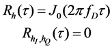
According to [1], when receiver moves relatively to the transmitter in a uniform scattering environment, Doppler shift will occur, which makes correlation functions of satisfy:

(1)

where is the maximum Doppler frequency. and are the real and imaginary parts of respectively and they are independent. is the zero-order Bessel function of the first kind and its Fourier transform (2) is the power spectral density (PSD) of, which is called the Jakes Doppler spectrum [1].

(2)

Channel simulator is designed to generate the fading process whose correlation functions and PSD satisfy (1) and (2) respectively. In the open literature, two methods have been proposed to design the simulator.

The first method, called “the sum of sinusoids”, was first proposed by Jakes [2], where a number of sine waves were summed up to simulate the fading process. Though the method is simple and easy to be implemented, fading process generated by this method lacks of randomness and some of its high order statistic characteristics are difficult to be consistent with theoretical ones [3].

The second method is to filter noise, where complex white Gaussian noises pass through a filter to generate the fading process. This filter, which we call Doppler filter, can be implemented by both FIR [4] and IIR filter [5]. Since the transition band is very steep in Jakes PSD (2), if using FIR filter to approximate it accurately, filter order needs to be high, which is expensive in terms of hardware resources. The IIR filter, however, can achieve excellent approximation with considerably low order.

Reference [5] proposed a simulator structure consisting of an IIR filter and an interpolator. It calculated coefficients of IIR filter using ellipsoid algorithm (EA) [6]. To keep the filter stable, any pole gone out of the unit circle in iterations would be reflected back. This makes the iteration start from a new point, like random searching.

Reference [7] [8] also used EA but proposed a barrier function to constrain poles lying inside the unit circle. However, the convergence will be affected by the starting point, because non-convexity of the problem. To the best of my knowledge, previous articles used cascaded low order IIR filter only mentioned the non-convexity of their objective functions, however, without proving.

Based on the review above, this article realizes a channel simulator proposed in [5] using different algorithm. We focus on the design of Doppler filter inside it, which is actually an IIR filter fitting problem. Non-convexity of the problem is proved for the first time and genetic algorithm is used to solve it, which is a kind of global optimization method and performs well in solving non-convex problems.

This paper is organized as follows. Section 2 introduces the structure of the channel simulator and defines the optimization problem to design the Doppler filter. Section 3 uses genetic algorithm to solve the problem and section 4 testifies correlation functions and LCR of the fading process generated. Finally, Section 5 concludes the paper.

Notation: The following notations are used throughout this paper. Boldface lowercase letter denotes vectors. Operator denotes the absolute value and represents Euclidean norm of vector. The superscript and denote complex conjugation and transposition respectively.

2. Channel Simulator

2.1. Structure of the Simulator

Figure 1 shows the structure of the channel simulator used in this paper, which consists of three parts. Noise generator produces complex white Gaussian noise. Doppler filter filters white noise to generate correlated noise with its PSD complying with Jakes PSD. Interpolator makes Doppler rate of the fading process output satisfy the requirement of the physical channel. The Doppler rate is defined as, where is the sampling rate of fading process [5].

The value at the Doppler filter usually takes 0.2. When implemented, Doppler filter remains unchanged and interpolation factor of the interpolator is changed to adjust at the output:. This article will focus mainly on the design of the Doppler filter next.

One important consideration in designing Doppler filter is to ensure the stability. Generally, the larger the filter order is, the more difficult to keep it stable. On account of this, a good choice is to use the cascaded low order IIR sections as the Doppler filter. Except for being easy to be stable, this structure has additional advantage that is less sensitive to quantization error compared with high order IIR filter.

Formula (3) shows the system function of the traditional biquad IIR filter, where a, b, c, d are real-valued optimization variables. Reference [9] studied the stable condition of this biquad, which was called the “Triangle Stability Region” but not intuitive.

(3)

We factorize its numerator and denominator, writing it into the form of conjugate poles and zeros (4), where zr, zi, pr and pi are real-valued optimization variables, representing the real and imaginary parts of zero and pole respectively.

(4)

This Second-Order Section (SOS) is inherently stable, as long as all poles are strictly inside the unit circle. When implementing in a physical system, restore

the conjugate form into its traditional biquad form.

(5)

Usually, multiple of SOSs need to be cascaded to approximate the objective response. Assuming we use SOSs, and uniformly sample variable into points points along the unit circle: (usually M = 500), to get the frequency response of Doppler filter after frequency sampling:

(6)

wherein is the scaling factor and is a vector containing all optimization variables:

(7)

2.2. Optimization Model

Ideal amplitude response of Doppler filter is the square root of Jakes PSD (2) but cannot be realized with a physical system according to Paley-Winner theorem, because at the frequency point the amplitude of Jakes PSD changes from into zero immediately. For this reason, [4] gives a modified objective response that can be achieved by a stable system. Referring to it herein, this article uses (8) as the objective amplitude response, where is the index of frequency point.

(8)

In the formula above, parameter SA denotes the stopband attenuation relative to the passband. Objective function could be defined as:

(9)

where is a weight vector to emphasize the error minimization for certain frequency band [7]. The complete optimization problem is:

(10)

wherein constraint is an empirical condition. limits poles of the SOS located inside the unit circle to keep Doppler filter stable. Constraint confines zeros lying inside the unit circle too, so that the Doppler filter will be a minimum phase system and have the minimum group delay.

Non-convexity of (10) confirms only if one point exists in the feasible region, around which the objective function is not convex. We will find such next.

According to the first-order conditions of convexity, is convex if and only if the feasible region () is convex and (11) holds for all [10].

(11)

Here denotes the gradient of respect to, and is the incremental step of.

For problem (10), is obviously a convex set. To show the non-con- vexity of, we randomly generate from and approximately calculate using its finite difference in computer. Then change gradually and plot and its first-order approximation to see if equation (11) is satisfied.

An example is showed in Figure 2, in which we see that is not convex around. Indeed, much more than one points like could be found in simulation, at which is not convex.

3. Genetic Algorithm

3.1. Introduction of Genetic Algorithm

Genetic Algorithm (GA) simulates the evolution process of biotic population with selection, crossover and mutation operations. The population evolves after several generations to achieve a stable situation, which corresponds to the convergence of optimization problem [11]. Procedures in simulating GA have been described as pseudocodes in Figure 3.

Some terminologies of GA will be used in the subsequent content: A possible solution of the optimization problem is called an individual in GA. Each individual consists of a number of genes and each gene corresponds to an optimization variable. For example in (7) is called an individual, and variables A, zr, zi, pr and pi in are genes. Technical details of the pseudocodes will be given in the following.

3.2. Solving the Problem Using GA

GA parameters: Supposing that Doppler filter uses K = 7 cascaded SOSs, the referenced GA parameters are listed in.

Table 1. Generally, the larger Nind is, the greater probability that the global optimal solution may be contained in the population, so Nind should be configured big enough to keep a good diversity of the genes.

Initializing population: This step generates the initial population and each member must be feasible, meaning that individuals must satisfy constraints in (10). Firstly, generate genes A, zr, zi, pr and pi from uniform distribution in the range [−1, 1] as an individual.

(12)

Then checking the feasibility, add the individual into the initial population if its poles and zeros are all within the unit circle, otherwise discard. Repeat this process until Nind feasible individuals are created to form an initial subpopulation.

Calculating fitness: Fitness is used to quantitatively describe each individual’s adaption to the environment. This article chooses the value of objective function as fitness and the value smaller represents better adaptation.

(13)

In this step, compute the objective function value of individuals in each subpopulation first, then sort all individuals in an ascend order according to their fitness values.

Selecting elite individuals: Elite individuals refer to those who have the best adaptabilities in every subpopulation. They are preserved and passed to the next generation directly, which ensures that the performance of the new population will not degrade. This step selects Nelite individuals in each subpopulation, whose objective function values are smallest.

(14)

Selection: Selection is to select Nparent individuals from each subpopulation to produce offspring. Individuals stronger will have more opportunities to be selected and mate, while those with poor adaptability will be eliminated gradually. All individuals selected will be divided into two parts, where the first part will do crossover operation, and another part will mutate. In crossover, individuals need to be selected as parents because two parental individuals will produce one child. As for mutation, Nmut parents are needed because one single parent mutates to produce one child.

In this paper, a tournament selecting method [12] has been used. S (tournament size, e.g. 4) players are randomly chosen from each subpopulation in the tournament. A player is an individual and the one that has the best fitness value will be selected. Repeat this process until Nparent parental individuals are selected in each subpopulation.

Crossover: Crossover simulates the mating process of natural population. In the operation, parental individuals are paired first and each pair consists of a father and a mother. Then randomly select half of genes from the father, and the complementary half from the mother. Finally combine these two parts of genes together to produce a child.

(15)

The subscript is the index of gene in the individual and rnd is a random integer generated from 0 and 1. Totally Nxov children in each subpopulation are need to be produced in this step.

Mutation: In a biotical population, gene mutation happens when passing genes from parents to children, which will produce new genes and increase the genetic diversity of the population. Gaussian mutation [13] is one kind of classical mutation methods in GA, where a random variable, generated from the Gaussian distribution (16) with zero mean and standard variance, will be superimposed on the original gene as a mutation variation.

(16)

At the beginning of the GA, each gene is dispersedly distributed in the entire feasible region. The variation magnitude can be relatively big at this moment to offer more possibilities for each gene. However, as the evolution progresses, each gene begins to converge and variation magnitude should be reduced accordingly. Because after evolution, gene values that were far away from their values, now have been eliminated already by natural selection. If the variation amplitude generated is too large, the gene newly mutated will still be eliminated with great probability in the subsequent evolution, which indicates that such mutation has no meaning.

This article chooses the standard variance of to be of the Gaussian distribution. As the iteration progresses, will gradually converge, tracking this tendency becomes smaller. Thus the variation magnitude will also decrease, which avoids invalid searching.

Combination: After mutation, all offspring have been produced and they will be combined to generate a new population, which consists of three parts. The first one is the elite individuals retained from the population of the last generation. The second one is the offspring created by crossover operation and the last part is the children generated by mutation, whose genes are mutated versions of their parents’ genes.

Population newly generated will be delivered to calculate fitness again and the generation number Gen will be updated. So the evolution continues and optimization variables converge to the global or near global optimum solution gradually.

Migration: Migration occurs every MigG generations past promoting the communication between subpopulations. Elites of each subpopulation are gathered up first in this step, then they are randomly divided into Nsub parts, passed to each subpopulation to replace their worst fit individuals. Subpopulation and migration mechanism can efficiently improve the probability of getting the global optimal in GA.

4. Simulation Results

Simulating GA described above in Matlab, we get the Doppler filter. Figure 4 shows the amplitude response of the designed Doppler filter. We see that it matches closely with the targeted response in passband, the transition band is very sharp and the response in stopband fluctuates slightly around.

There are two criterions to measure the statistical accuracy of fading channel simulator. The first one is the correlation function. As an example, Figure 5 shows the correlation characteristics of the generated fading process and we see that both auto-correlation and cross-correlation functions simulated match well with theoretical curves.

Another statistic characteristic of the fading channel is the LCR, which indicates the speed of the envelope of passing through level in the downward direction. For Rayleigh fading channel, LCR satisfies (17), where is the signal level being crossed normalized with the rms of the fading process [1].

(17)

Figure 6 shows the simulated LCRs, which are in good agreement with theo-

retical ones, expect for two situations where the LCR values are underestimated. However, according to [5], these situations are common problems and unrelated to the particular simulation techniques used. We see that mismatches disappear as interpolation factor increases.

5. Conclusion

This paper designs the channel simulator producing correlated Gaussian noises as the Rayleigh fading waveforms. An optimization model has been built to design the Doppler filter, and its non-convexity is proved with the aid of computer simulation. Genetic algorithm is used to solve the problem and it converges to the solution corresponding to very accurate approximation of Jakes PSD. Also statistical characteristics of the generated fading process match well with theoretical predictions, which confirms the validity of the simulator we designed.

Cite this paper

Wang, H.F., Du, S.W. and Guan, N. (2017) Design of Fading Channel Simulator Based on IIR Filter Using Genetic Algorithm. Int. J. Communications, Network and System Sciences, 10, 105-115. https://doi.org/10.4236/ijcns.2017.105B010

References

- 1. Goldsmith, A. (2005) Wireless Communications. Cambridge University Press, Cambridge, 71-82. https://doi.org/10.1017/cbo9780511841224
- 2. Jakes, W.C. and Cox, D.C. (1994) Microwave Mobile Communications. Wiley IEEE Press. https://doi.org/10.1109/9780470545287
- 3. Pop, M.F. and Beaulieu, N.C. (2001) Limitations of Sum-of-Sinusoids Fading Channel Simulators. IEEE Transactions on Communications, 49, 699-708. https://doi.org/10.1109/26.917776
- 4. Young, D.J. and Beaulieu, N.C. (2000) The Generation of Correlated Rayleigh Random Variates by Inverse Discrete Fourier Transform. IEEE Transactions on Communications, 48, 1114-1127. http://doi.org/10.1109/26.855519
- 5. Komninakis, C. (2003) A Fast and Accurate Rayleigh Fading Simulator. GLOBECOM’03, IEEE Global Telecommunications Conference, 6, 3306-3310. https://doi.org/10.1109/GLOCOM.2003.1258847
- 6. Boyd, S. and Barratt, C. (2008) Ellipsoid Method. Notes for EE364B, Stanford University.
- 7. Alimohammad, A., Fard, S.F. and Cockburn, B.F. (2012) Filter-Based Fading Channel Modeling. Modelling and Simulation in Engineering, 2012, 3. https://doi.org/10.1155/2012/705078
- 8. Alimohammad, A. and Fard, S.F. (2013) Fpga Implementation of Isotropic and Noniso-tropic Fading Channels. IEEE Transactions on Circuits and Systems II: Express Briefs, 60, 796-800. https://doi.org/10.1109/TCSII.2013.2281768
- 9. Lu, W.-S. and Hinamoto, T. (2003) Optimal Design of Iir Digital Filters with Robust Stability Using Conic-Quadratic-Programming Updates. IEEE Transactions on Signal Processing, 51, 1581-1592. https://doi.org/10.1109/TSP.2003.811229
- 10. Boyd, S. and Vandenberghe, L. (2004) Convex Optimization. Cambridge University Press, 69-70. https://doi.org/10.1017/CBO9780511804441
- 11. Chipperfield, A., Fleming, P., Pohlheim, H. and Fonseca, C. (1994) Genetic Algorithm Toolbox for Use with Matlab.
- 12. Filipovic, V. (2012) Fine-Grained Tournament Selection Operator in Genetic’ Algorithms Computing and Informatics, 22, 143-161.
- 13. Higashi, N. and Iba, H. (2003) Particle Swarm Optimization with Gaussian Mutation. Proceedings of the 2003 IEEE Swarm Intelligence Symposium, SIS’03, 72-79. https://doi.org/10.1109/SIS.2003.1202250