Intelligent Control and Automation
Vol. 3 No. 3 (2012) , Article ID: 22050 , 11 pages DOI:10.4236/ica.2012.33029
Observer-Based Nonlinear Feedback Controls for Heartbeat ECG Tracking Systems
Center for Robotics and Advanced Automation, Oakland University, Rochester, USA
Email: tporntha@oakland.edu, loh@oakland.edu
Received June 10, 2012; revised July 9, 2012; accepted July 16, 2012
Keywords: Heartbeat Model; Electrocardiogram; Nonlinear Control of Biological Systems; Input-Output Feedback Linearization; Observer-Based Nonlinear Control Systems
ABSTRACT
The analysis and design of observed-based nonlinear control of a heartbeat tracking system is investigated in this paper. Two of Zeeman’s heartbeat models are investigated and modified by adding the control input as a pacemaker, thereby creating the control-affine nonlinear system models that capture the general heartbeat behavior of the human heart. The control objective is to force the output of the heartbeat models to track and generate a synthetic electrocardiogram (ECG) signal based on the actual patient reference data, obtained from the William Beaumont Hospitals, Michigan, and the PhysioNet database. The formulations of the proposed heartbeat tracking control systems consist of two phases: analysis and synthesis. In the analysis phase, nonlinear controls based on input-output feedback linearization are considered. This approach simplifies the difficult task of developing nonlinear controls. In the synthesis phase, observer-based controls are employed, where the unmeasured state variables are estimated for practical implementations. These observerbased nonlinear feedback control schemes may be used as a control strategy in electronic pacemakers. In addition, they could be used in a software-based approach to generate a synthetic ECG signal to assess the effectiveness of diagnostic ECG signal processing devices.
1. Introduction
The human heart is a complex yet robust system. One of the most important signals that are being generated during the operation of the human heart is the electrocardiogram (ECG). It is a time-varying signal measuring the potential of the electrical activities in the cardiac tissue. A single cycle of the ECG consists of the contraction and relaxation of the heart, which is the heart pumping action. The ECG can be measured by recording the potential differences between two electrodes placed on the skin at pre-determined positions. The characteristic information extracted from the ECG can be used to assess the state of the cardiac health and potential heart problems [1,2].
The research and development of mathematical models for heartbeats or heart rhythms have been very active in the literature [3-17]. One of the important developments was accomplished by Zeeman [3], where the models captured, at least qualitatively, three essential characteristics of the cardiac dynamics: 1) a stable equilibrium; 2) a threshold for triggering the action potential; and 3) the return to equilibrium. The resulting models are a 2nd- order nonlinear ordinary differential equation (ODE) of the Liénard-type representing the heartbeat dynamics, and a 3rd-order nonlinear ODE that can be applied to the nerve impulse. These models are based on the normal pacemaker generated by the sino-atrial (SA) node [4], which is the dominant pacemaker as compared to the slower one produced by the atrio-ventricular (AV) junction. This slower pacemaker is regarded in [5] as a passive conduit. In [6], the authors modified the 2nd-order ODE heartbeat system in [3] by incorporating an on-off control variable representing the pacemaker mechanism of contraction-relaxation of the heart. Reference [7] modified the 3rd-order nonlinear ODE model in [3] by adding control parameters that affect the frequency of the oscillation to control the heart rate variability and used a neural network to produce the ECG signal.
Another well-known approach to modeling the cardiac induction system is based on the van der Pol (VdP) type oscillators [8]. The idea of this approach stems from the analogy between the properties of relaxation oscillators and those of biological pacemakers. In contrast to [3], a coupled VdP oscillator assumes a more active role for the AV pacemaker, and considers the coupling effect between the SA and the AV pacemakers in the normal electrophysiological dynamics. A study of the synchronization properties of the rhythms produced by the SA and AV nodes using two coupled VdP oscillators was investigated in [9-13]. Furthermore, reference [14] proposed a proportional feedback control algorithm to synchronize the rhythm of the SA and AV pacemakers using the model from [11,12]. Recently, Gois and Savi [15] proposed a heart rhythm model that consists of three coupled modified VdP oscillators with time delay. Numerical simulations were carried out to reproduce the ECG signal that could be altered by changing the coupling parameters. A dynamical model that generates a synthetic ECG signal, based on statistical information such as the mean, standard deviation of the heart rate, and the power spectrum of the RR tachogram was proposed in [16]. The model does not rely on the dynamics of the heart but the ECG statistical information as a priori data to generate the signal. Reference [17] studied the synchronization between the models from [15,16] as a tracking control problem by using the model from [15] as a process plant and the ECG generated by the model from [16] as a reference signal, and proposed a heart rhythm proportional controller with  tracking error as one of the control parameters.
This paper considers the analysis and design of observer-based controls of the modified Zeeman’s models in [3] using the input-output feedback linearization technique. A previous investigation without observers was presented in [18]. Observer-based techniques and technology are motivated by the needs of practical implementations: for systems with inaccessible state variables, it will be difficult to implement most control schemes requiring feedback of the inaccessible states without an observer for state estimation. An observer-based control scheme is, in general, more difficult to analyze and design. The importance of the observer-based nonlinear feedback tracking control technique developed in this paper is that it may be used as a control strategy for electronic pacemakers, or a software-based generation of a synthetic ECG signal for assessing the effectiveness of diagnostic ECG signal processing devices.
The paper is organized as follows. In Section 2, the dynamic model and its characteristics are investigatedphase portraits and stability analysis are conducted. Section 3 provides the fundamental of nonlinear feedback linearization control and observer theory. The results of the observer-based nonlinear tracking control systems and the simulation results are demonstrated in Section 4. The conclusions are presented in Section 5.
2. The Heartbeat Models
A cycle of the heartbeat consists of two states: diastole which is the relaxed state, and systole which is the contracted state. The cycle starts when the heart is in the diastolic state. The pacemaker that is located at the top of the right atrium—one of the upper chambers of the heart —triggers an electrochemical wave that spreads slowly over the atrium. This electrochemical wave causes the muscle fibers to contract and push the blood into the ventricles—the lower chambers of the heart. The electrochemical wave then spreads rapidly over the ventricles causing the whole ventricle to contract into the systolic state, and pumping the blood into the lung and the arteries. Immediately following the systolic state, the muscle fibers relax quickly and return the heart to the diastolic state to complete one cycle of the heartbeat [6].
A mathematical model that describes the behavior of the heartbeat was developed in [3], where it was suggested that such a model should contain three basic features:
1) A stable equilibrium state representing diastole;
2) A threshold for triggering the electrochemical wave causing the heart to go into systole; and 3) The return of the heart to the diastolic state.
The resulting models that address the characteristics above are given below.
2.1. The 2nd-Order Nonlinear Heartbeat Model
The 2nd-order nonlinear heartbeat model is given by
 (1)
(1)
where  represents the length of the muscle fiber,
  is a variable related to electrochemical activities, and can be measured as the potential across the membrane of the muscle fiber—the ECG signal; the parameter
 ![]() is a small positive constant associated with the fast eigenvalue of the system,
is a small positive constant associated with the fast eigenvalue of the system,  is a scalar quantity representing a typical length of muscle fiber in the diastolic state, and
  represents tension in the muscle fiber.
Figure 1 illustrates the phase portrait of (1) with the initial conditions along the left and right diagonals across the  plane. The parameter values used to produce the phase portrait are
 , T = 1, and
  The cubic line (dashed curve) represents the steady-state of the first equation in (1). When
 , the equilibrium point of the system is at the origin. All trajectories initiated above the cubic line, i.e.,
  direct downward toward the origin along the cubic line.
Likewise, all trajectories started below the cubic line, that is,  , direct upward toward the origin along the cubic line. All trajectories end up at the limit cycle around the equilibrium point. It is obvious that the equilibrium point is unstable as the vector field inside the limit cycle directs away from the point. This conclusion can be affirmed by analyzing the stability of the equilibrium point using the well-known Lyapunov indirect stability theorem [19]. For this purpose, let A be the constant Jacobian matrix of (1) at the origin, it fol-
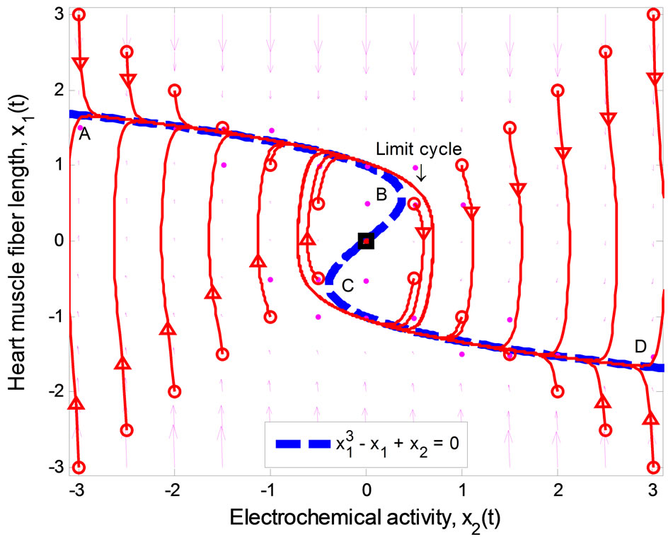
Figure 1. Phase portrait of the 2nd-order heartbeat system for ε = 0.2, T = 1, xd = 0.
lows that
 (2)
(2)
The eigenvalues of A are given by  and
and  for
for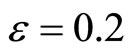 , and
, and  therefore, the origin is unstable since both eigenvalues are real and positive.
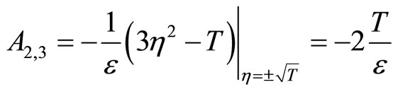
In Figure 1, since the vector field around the segment AB and CD always points toward the cubic line, and away from the cubic line in the BC portion, any point along the cubic line in the AB and CD segments is considered to be stable whereas points along the BC section are unstable. The points B and C are important as they specify the threshold—the second basic feature (ii) of the heartbeat model mentioned earlier. These points can be computed easily by considering the eigenvalues of the matrix A in (2)
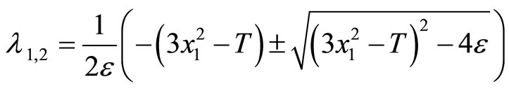 (3)
(3)
The condition that the real part of the eigenvalue is negative is . Therefore, the system is stable if
  which refers to the section AB, and
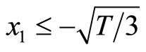 which describes the section CD. In other words, the thresholds for switching between the diastolic and the systolic states at point B is
 , and
, and  at point C.
The stable equilibrium point that represents the state of diastole can be determined by changing the value of  in the second equation of (1) such that it satisfies the stability condition above. Figure 2 displays the phase portrait of the system with
 . The equilibrium point is stable at (1.024, −0.0497), and qualifies to be the
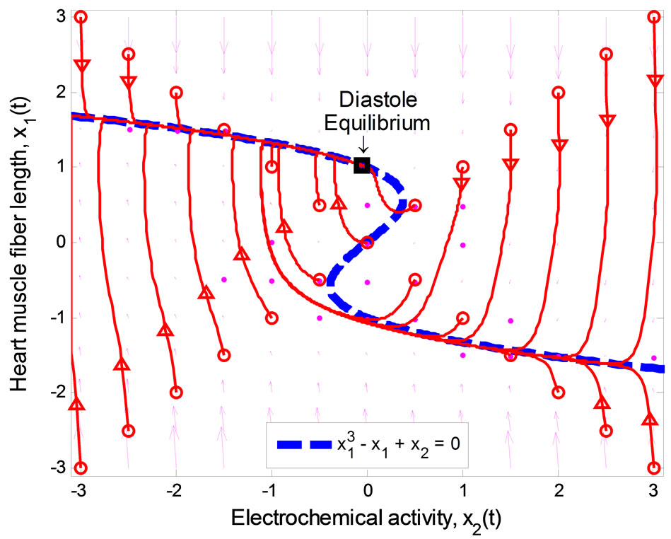
Figure 2. Phase portrait of the 2nd-order heartbeat system during diastole for ε = 0.2, T = 1, xd = 1.024.
diastolic equilibrium state, i.e., satisfies the first feature (i): a stable equilibrium.
In Figure 2, all of the trajectories, regardless of their initial condition, end up at the diastolic equilibrium point. Since the equilibrium point is stable, the system will stay at this point forever unless there is an external excitation that forces the system to a new equilibrium point. In [6], the authors modified the system by adding a control input u(t) as shown below:
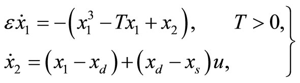 (4)
(4)
where the additional parameter  represents a typical fiber length when the heart is in the systolic state, and
  represents the cardiac pacemaker control mechanism that directs the heart into the diastolic and the systolic states. By setting the cardiac pacemaker control signal u(t) in the form of {0} and {1} (on-off controls), the equilibrium point of the system can be switched between the diastolic and the systolic states. Figure 3 displays the phase portrait with
  the stable equilibrium point is located at (−1.3804, 1.25).
2.2. The 3rd-Order Nonlinear Heartbeat Model
The 3rd-order nonlinear heartbeat model is given by
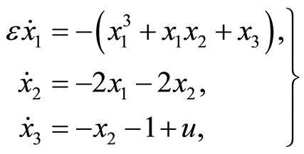 (5)
(5)
where  refers to the length of the muscle fiber,
  represents tension in the muscle fiber,
  is related to electrochemical activities,
 ![]() is a positive constant, and u(t) represents cardiac pacemaker control
is a positive constant, and u(t) represents cardiac pacemaker control

Figure 3. Phase portrait of the 2nd-order heartbeat system during systole for ε = 0.2, T = 1, xd = –1.3804.
signal which directs the heart into the diastolic and the systolic states.
The dynamics of the 3rd-order system are similar to those of the 2nd-order system except that the dynamic of the muscle fiber tension is taken into consideration, that is, the constant T in the 2nd-order system becomes a state variable  in the 3rd-order system.
3. Theoretical Background
3.1. Nonlinear Input-Output Feedback Linearization
Consider a control-affine single-input single-output (SISO) nonlinear system described by
 (6)
(6)
where  is the state vector,
  are the control and output, respectively; f, g are smooth vector fields in a domain D and h a smooth function in D, where D is an open set in
Given the nonlinear system in (6), our goal is to find a transformation function (diffeomorphism)  with
with  that transforms the nonlinear system in the x-coordinates to a linear system in the z-coordinates. One of the most important reasons for finding the transformation is that the powerful linear system theory and methodologies can be applied once a nonlinear system has been linearized.
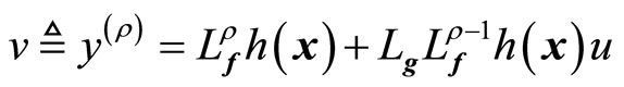
Differentiating the output  with respect to t yields
 (7)
(7)
where  and
and  denotes the Lie derivatives of
  with respect to
  and
and , respectively. If
 , then
  is not a function of
 . Continuing successive differentiation ρ times until the input
  appears explicitly, we obtain
 (8)
(8)
The smallest integer  for which u(t) appears is referred to as the relative degree. The nonlinear system in (6) is said to have a well-defined relative degree
  in a region
  if
if ,
, ; and
; and ,
, . When the relative degree is equal to the dimension of the nonlinear system, that is,
  , the system is said to be fully linearizable, whereas it is only partially linearizable if
  (both heartbeat systems considered in Section 4 below have
 ; hence both are partially linearizable).
From (8), we define
 (9)
(9)
where v(t) is a one-dimensional transformed input created by the feedback linearization process. Equation (9) yields the linearizing feedback control law [19-21]
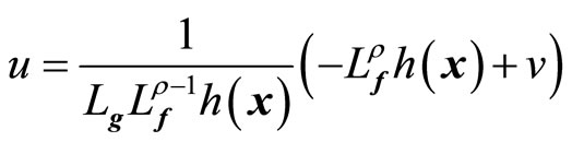 (10)
(10)
provided  is nonsingular.
To develop an overall representation of the system for the partially linearized case with , the transformation function
  can be expressed as
 (11)
(11)
where ,
,  and
and  are chosen such that
  is a diffeomorphism in a domain
 . In other words, the Jacobian matrix associated with
  is nonsingular, and
 (12)
(12)
for all .
.
The transformation (11) leads to the normal form [20]
 , (13)
 , (14)
 (15)
(15)
where  and
and  are in controllable canonical forms given by, respectively,

Equation (13) represents the external dynamics, while (14) is referred to as the internal dynamics of (6). Setting  in (14) for all
  yields
 (16)
(16)
which represents the zero dynamics for (6). The stability of the zero dynamics in (16) is an important issue in designing a controller. A system whose zero dynamics are asymptotically stable in the domain of interest is called a minimum phase system. The local asymptotic stability of the zero dynamics is, clearly, the necessary and sufficient conditions for the local asymptotic stability of the feedback linearized system described in (13)-(15) [21,22]. In the case that the zero dynamics are unstable in the region of interest, the system is known as a non-minimum phase system. Generally, a system of this type cannot be used for state-feedback control system design because some of the state variables will escape to infinity. In this case, the stabilization of the unstable zero dynamics needs to be considered, if possible.
3.2. Asymptotic Output Tracking
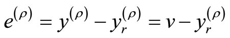
Let the control objective be steering the output  to a desired reference signal
 . This gives rise to an output tracking control problem. Defining the output tracking error as
 , the main objective is to force
  such that
  as
as . It follows that
 (17)
(17)
A suitable tracking control law for the transformed input v(t) is given by
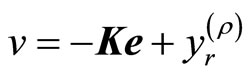 (18)
(18)
where ,
,  is the constant gain matrix to be determined such that
 is Hurwitz, that is, all of the eigenvalues of
  lie in the open left-haft complex plane. Combination of (18) and (10) yields the nonlinear tracking control law
 (19)
(19)
3.3. Observer for Normal Form
The design of observer-based nonlinear control system is addressed in this section to provide real-time estimates of the inaccessible dynamical states required for the implementation of control laws. It is well-known that a Luenberger observer for a nonlinear control system based on input-output feedback linearization when  exists, since the transformed system in the z-coordinates is in linear controllable canonical form. However, this is not true for the normal form, i.e., when
 , because the internal dynamics (14) are unobservable by the chosen output
  [19,20]. Nonetheless, by applying the results of [23,24], we will show that an observer for such systems may be possible. Without loss of generality, we assume that the normal form (13)-(15) has the equilibrium point at the origin. First, we linearize the normal form given by (13) and (14) in the following partitioned form:
 (20)
(20)
where ,
,  ,
,  ,
,  , z is given in (11), and where
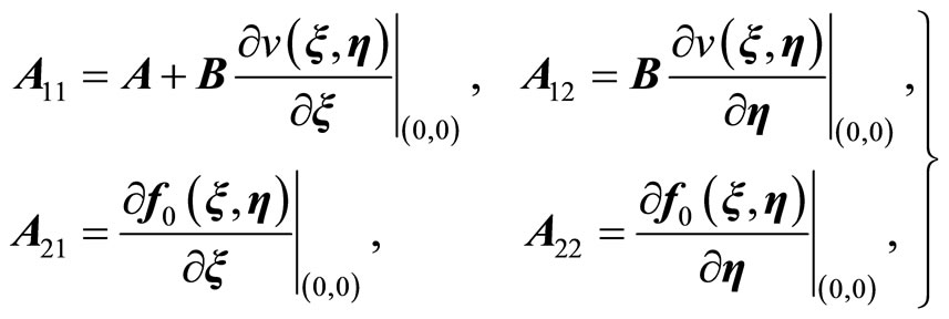 (21)
(21)
 (22)
(22)
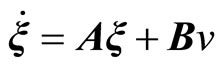
Equation (20) is in a standard linear system with  being considered as a disturbance vector. If
  is an observable pair, that is,
 (23)
(23)
and the term  is Lipschitz so that there exists a Lipschitz constant
  such that
 (24)
(24)
for all z in a region , then an observer for (20) can be formulated as
 (25)
(25)
where the gain matrix  is determined in such a way that
  is Hurwitz.
Now, let the estimation error associated with (20) and (25) be defined by . We need to show that
  converges to zero asymptotically. It follows from (20) and (25) that
 (26)
(26)
Consider a Lyapunov candidate function
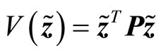 (27)
(27)
where P is a real symmetric positive definite matrix and is the solution of the Lyapunov equation
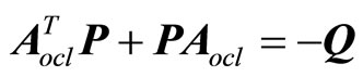 (28)
(28)
with Q a positive definite symmetric matrix. It follows that
 (29)
(29)
Since  is Lipschitz, so is
 . Substituting (24) into (29) yields
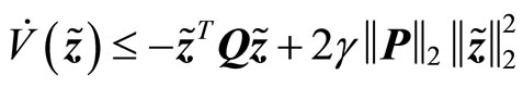 (30)
(30)
Since , it follows that
 (31)
(31)
is negative definite, provided , so that the estimation error
 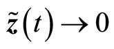 as
as .
.
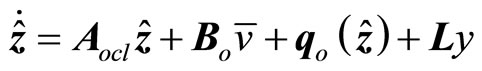
Finally, with reference to (11), the observer given by (26) can be expressed in the x-coordinates as
 (32)
(32)
4. Application to the Heartbeat Systems
We apply the theoretical results above to develop an observer-based nonlinear tracking control for the heartbeat systems (4) and (5). First, we consider the 2nd-order heartbeat system (4), with  as the output measurement (recall that
  can be measured as the potential across the membrane of the muscle fiber).
Differentiating the output with respect to t yields
 (33)
(33)
where u(t) appears, hence the relative degree is . The diffeomorphism T is given by
 (34)
(34)
where  satisfies (12). Equation (34) shows that the original system in (4) is already in a normal form when the output is chosen as
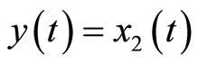 . We note that (34) reveals that
  and
and  are the internal and external dynamics, respectively. Rewriting (4) using (34) yields the normal form
 (35)
(35)
 (36)
(36)
 (37)
(37)
The zero dynamics satisfy
 (38)
(38)
There are three equilibrium points for (38): ,
, . We need to analyze the stability of the zero dynamics. Applying the Lyapunov indirect stability theorem [19] to (38), the Jacobian matrices at the origin and
  are given by
 (39)
(39)
 (40)
(40)
Since T and ![]() are positive constants, it follows that
are positive constants, it follows that  and
and , hence the equilibrium point at the origin is unstable and the equilibrium points at
  are asymptotically stable. In other words, regardless of the unstable equilibrium at the origin, the steady-state of the zero dynamics will end up at either the point
  or
or  depending on the initial condition. As a result, the zero dynamics are asymptotically stable. Therefore, the 2nd-order heartbeat system is a minimum-phase system.
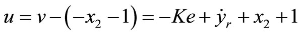
To proceed to the output tracking control design, we let the tracking error be  where
where . Using (18), the transformed input v(t) is given by
 (41)
(41)
where K = 100 is obtained by placing the real pole at s = –100 of the complex plane. Consequently, the linearizing feedback control law according to (19) is given by
 (42)
(42)
The development of an observer is accomplished by rewriting (35)-(37) in the form of (20) as:
 (43)
(43)
where . It follows that
  in (43) is observable, and the term
  is locally Lipschitz. Therefore, the observer for (43) is given by (25) where the gain matrix
  is chosen by placing the observer poles at
  of the complex plane. Finally, the observer-based tracking control law for the 2nd-order heartbeat system is given by
 (44)
(44)
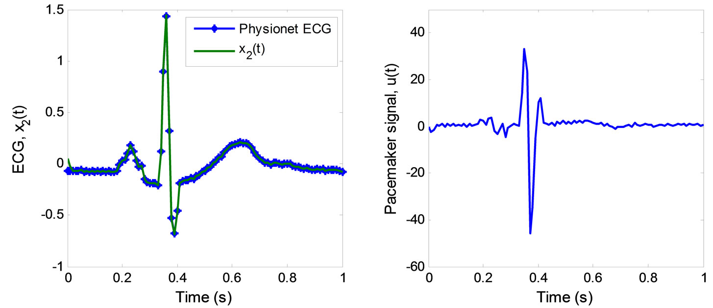
The simulation of the 2nd-order heartbeat control system (4) with the output  and the control law (44) was conducted using MATLAB. Figure 4 displays the tracking result of real discrete ECG data from PhysioNet database [25]. In Figure 4(a), the output
  converges and tracks the ECG reference signal very well. Figure 4(b) displays the pacemaker signal or the control law described in (44).
Figure 5 demonstrates the result of the observer in the x-coordinates along with the estimation errors. The initial condition of  is
is , and that of the estimated states
  is (0, 0). Both estimated states converge quickly to the real states, especially
 . Finally, the multiple pulses ECG signal is illustrated in Figure 6.
Next, consider the 3rd-order heartbeat system (5) with  as the output measurement. Differentiating the output with respect to t yields
 (45)
(45)
The relative degree is . We obtain the transformation function
 (46)
(46)
which also shows that the original system (5) is already in a normal form when the output is . Note that
  and
and 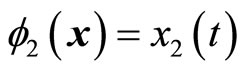 satisfy (12). The normal form is written as
 (47)
(47)
 (48)
(48)
 (49)
(49)
 (50)
(50)
The zero dynamics are given by
 (51)
(51)
There are two equilibrium points associated with (51): the origin, and  = (1,–1). Applying the Lyapunov indirect stability theorem [19] to the latter equilibrium point yields
 . (52)
It follows that  where
where  represents the
  eigenvalue; hence, matrix
  is Hurwitz. Therefore, the equilibrium point at (1, –1) is asymptotically stable. Next, consider the equilibrium point at the origin
 (53)
(53)
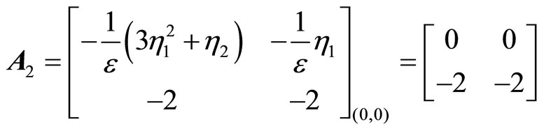
The eigenvalues of  are 0 and –2. Since one of the eigenvalues is zero, we cannot draw the stability conclusion by the Lyapunov indirect stability theorem. However, using the application of the center manifold theory [19] to determine the stability of the equilibrium point at the origin by analyzing a reduced-order system—a system whose order is exactly equal to the number of the
 (a) (b)
Figure 4. ECG tracking simulation results for the 2nd-order heartbeat system. (a) ECG tracking; (b) Pacemaker signal.

Figure 5. Observer simulation results and the estimation errors.
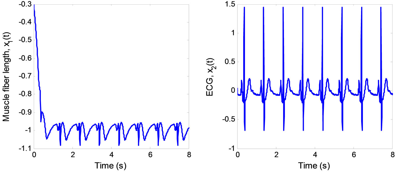
Figure 6. ECG signal produced by the 2nd-order heartbeat tracking system.
eigenvalues of  with zero real part, we found that the equilibrium point at the origin is asymptotically stable. This conclusion is illustrated by the phase portrait of the zero dynamics (51) as shown in Figure 7. All trajectories with initial condition
  converge to the origin. We conclude that the normal form system in (47)-(50) is a minimum-phase system.
We proceed to the output tracking control design. Since the relative degree in this case is the same as in the 2nd-order case, the transformed control law v(t) is of the same form as in (41). Subsequently, the tracking control law is given by
 (54)
(54)
Similar to the 2nd-order case, the normal form (47)-(50) can be expressed in the form of (20) as
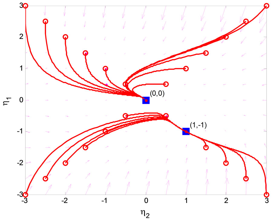
Figure 7. Phase portrait of zero dynamics of the 3rd-order heartbeat system.
 (55)
(55)
where . It follows that
  in (55) is an observable pair, and the term
  is locally Lipschitz. Thus, the observer for (55) is given by (25) where the gain matrix
  is obtained by placing the observer poles at
  of the complex plane. Finally, the observer-based tracking control law for the 3rd-order heartbeat system is given by
 (56)
(56)
The simulation result for the ECG tracking is shown in Figure 8(a) with the control pacemaker signal displays in Figure 8(b). The results show an effective output tracking of the discrete ECG data from the William Beaumont Hospitals, Michigan.
Figure 9 displays the real and estimated state of  to
to  including their estimation errors. It shows that the estimated states converge quickly to the
 (a) (b)
Figure 8. ECG tracking simulation results for the 3rd-order heartbeat system. (a) ECG tracking; (b) Pacemaker signal.

Figure 9. Observer simulation results and estimation error for the 3rd-order heartbeat system.
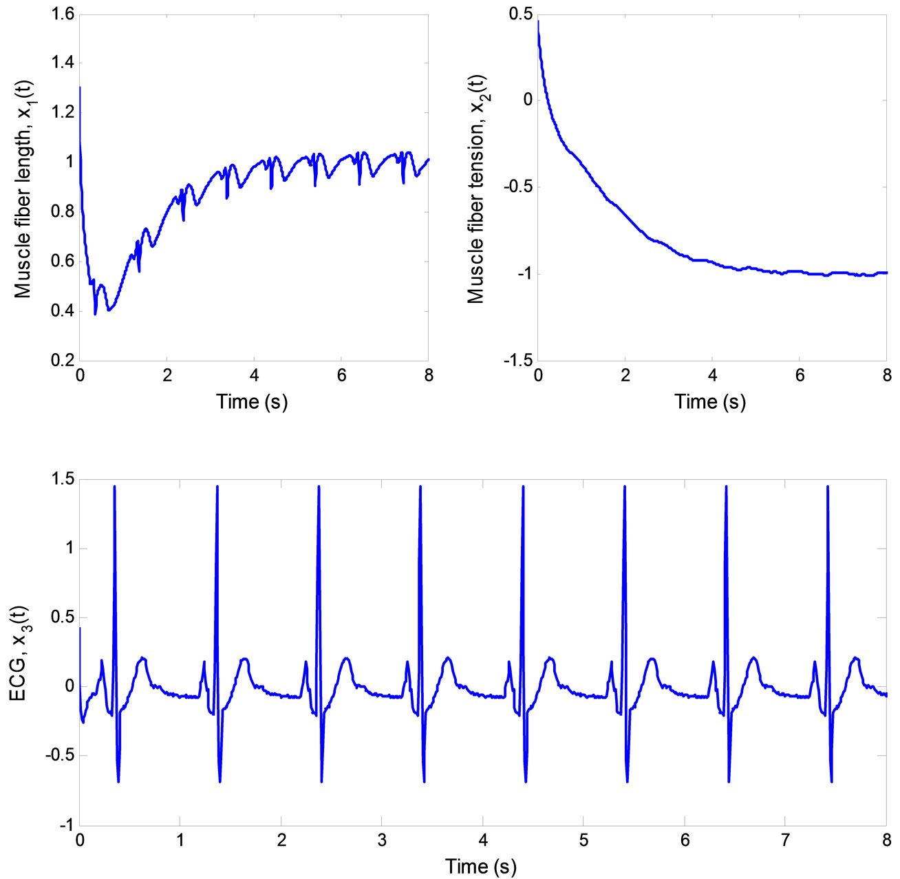
Figure 10. ECG signal produced by the 3rd-order heartbeat tracking system.
real states with asymptotically stable error dynamics. Finally, Figure 10 illustrates the multiple pulses ECG signal created by the 3rd-order heartbeat tracking system.
5. Conclusion
We applied the nonlinear control system theory, based on input-output feedback linearization and observer theory, to a model for the biological heartbeat systems. Two Zeeman models were chosen in this study as they not only describe the heartbeat, but also offer direct biophysical relationship to the dynamic variables. The two models were modified by incorporating a control input into the systems, thereby creating two interesting controlaffine SISO nonlinear systems. We showed that the resulting heartbeat models are minimum-phase systems suitable for the design of output tracking control laws; these control laws were also used to generate synthetic ECG signals. In addition, an observer was applied to estimate the unknown variables in the transformed coordinates. The simulation results show that the observerbased tracking control laws effectively force the outputs of the systems to track the real ECG data from the PhysioNet database (Figure 4), and William Beaumont Hospitals, Michigan (Figure 8), with asymptotic stable tracking error. Other biomedical engineering applications of Zeeman’s models are under consideration.
6. Acknowledgements
The authors wish to acknowledge the support of an Oakland University-Beaumont Hospital multidisciplinary research grant for biomedical engineering research under the Oakland University-William Beaumont School of Medicine. We would also like to thank Dr. Robert Hammond of the William Beaumont Hospitals, Royal Oak, MI, for providing a set of ECG data used in the simulation studies; Dr. Bradley Roth of the Department of Physics, and Dr. Edward Gu of the Department of Electrical and Computer Engineering, both at Oakland University, for their valuable comments and suggestions.
REFERENCES
- N. Kannathal, C. M. Lim, U. R. Acharya and P. K. Sadasivan, “Cardiac State Diagnosis Using Adaptive NeuroFuzzy Technique,” Medical Engineering & Physics, Vol. 28, No. 8, 2006, pp. 809-815. doi:10.1016/j.medengphy.2005.11.011
- L. Y. Shyu and W. Hu, “Intelligent Hybrid Methods for ECG Classification—A Review,” Journal of Medical and Biological Engineering, Vol. 28, No. 1, 2007, pp. 1-10.
- E. C. Zeeman, “Differential Equations for the Heartbeat and Nerve Impulse,” Towards a Theoretical Biology, Vol. 4, 1972, pp. 8-67.
- L. Glass, “Synchronization and Rhythmic Processes in Physiology,” Nature, Vol. 410, 2001, pp. 277-284. doi:10.1038/35065745
- M. Vassalle, “The Relationship among Cardiac Pacemakers: Overdrive Suppression,” Circulation Research, Vol. 41, No. 3, 1977, pp. 269-277. doi:10.1161/01.RES.41.3.269
- D. S. Jones and B. D. Sleeman, “Differential Equations and Mathematical Biology,” Chapman & Hall/CRC, London, 2003.
- N. Jafarnia-Dabanloo, D. C. McLernon, H. Zhang, A. Ayatollahi and V. Johari-Majd, “A Modified Zeeman Model for Producing HRV Signals and Its Application to ECG Signal Generation,” Journal of Theoretical Biology, Vol. 244, No. 2, 2007, pp. 180-189. doi:10.1016/j.jtbi.2006.08.005
- B. van der Pole and J. van der Mark, “The Heart Beat Considered as a Relaxation-Oscillation and an Electrical Model of the Heart,” Philosophical Magazine Series 7, Vol. 6, No. 38, 1928, pp. 763-775.
- B. J. West, A. L. Goldberger, G. Rovner and V. Bhargava, “Nonlinear Dynamics of the Heartbeat, the AV Junction: Passive Conduit or Active Oscillator?” Physica D: Nonlinear Phenomena, Vol. 17, No. 2, 1985, pp. 198-206. doi:10.1016/0167-2789(85)90004-1
- C. R. Katholi, F. Urthaler, J. Macy Jr. and T. N. James, “A Mathematical Model of Automaticity in the Sinus Node and AV Junction Based on Weakly Coupled Relaxation Oscillators,” Computers and Biomedical Research, Vol. 10, No. 6, 1977, pp. 529-543. doi:10.1016/0010-4809(77)90011-8
- M. G. Signorini, S. Cerutti and D. D. Bernardo, “Simulation of Heartbeat Dynamics: A Nonlinear Model,” International Journal of Bifurcation and Chaos, Vol. 8, No. 8, 1998, pp. 1725-1731. doi:10.1142/S0218127498001418
- D. D. Bernardo, M. G. Signorini and S. Cerutti, “A Model of Two Nonlinear Coupled Oscillators for the Study of Heartbeat Dynamics,” International Journal of Bifurcation and Chaos, Vol. 8, No. 10, 1998, pp. 1975-1985. doi:10.1142/S0218127498001637
- A. M. dos Santos, S. R. Lopes and R. L. Viana, “Rhythm Synchronization and Chaotic Modulation of Coupled van der Pol Oscillators in a Model for the Heartbeat,” Physica A: Statistical Mechanics and Its Applications, Vol. 338, No. 3-4, 2004, pp. 335-355. doi:10.1016/j.physa.2004.02.058
- M. E. Brandt, G. Wang and H. T. Shih, “Feedback Control of a Nonlinear Dual-Oscillator Heartbeat Model,” Bifurcation Control, Vol. 293, 2003, pp. 715-718.
- S. R. F. S. M. Gois and M. A. Savi, “An Analysis of Heart Rhythm Dynamics Using a Three-Coupled Oscillator Model,” Chaos, Solitons and Fractals, Vol. 41, No. 15, 2009, pp. 2553-2565. doi:10.1016/j.chaos.2008.09.040
- P. E. McSharry, G. D. Clifford, L. Tarassenko and L. A. Smith, “A Dynamical Model for Generating Synthetic Electrocardiogram Signals,” IEEE Transactions on Biomedical Engineering, Vol. 50, No. 3, 2003, pp. 289-294. doi:10.1109/TBME.2003.808805
- M. J. Lopez, A. Consegliere, J. Lorenzo and L. Garcia, “Computer Simulation and Method for Heart Rhythm Control Based on ECG Signal Reference Tracking,” WSEAS Transactions on Systems, Vol. 9, No. 3, 2010, pp. 263-272.
- W. Thanom and R. N. K. Loh, “Nonlinear Control of Heartbeat Models,” Journal on Systemics, Cybernetics and Informatics, Vol. 9, No. 1, 2011, pp. 21-27.
- H. K. Khalil, “Nonlinear Systems,” 3rd Edition, Prentice Hall, Upper Saddle River, 2002.
- A. Isidori, “Nonlinear Control Systems,” Springer-Verlag, New York, 1995.
- M. A. Henson and D. E. Seborg, “Nonlinear Process Control,” Prentice Hall, Upper Saddle River, 1997.
- C. I. Byrnes and A. Isidori, “Asymptotic Stabilization of Minimum Phase Nonlinear Systems,” IEEE Transactions on Automatic Control, Vol. 36, No. 10, 1991, pp. 1122- 1137. doi:10.1109/9.90226
- G. Ciccarella, M. Dallamora and A. Germani, “A Luenberger-Like Observer for Nonlinear Systems,” International Journal of Control, Vol. 57, No. 3, 1993, pp. 537- 556. doi:10.1080/00207179308934406
- N. H. Jo and J. H. Seo, “Input Output Linearization Approach to State Observer Design for Nonlinear System,” IEEE Transactions on Automatic Control, Vol. 45, No. 12, 2000, pp. 2388-2393. doi:10.1109/9.895580
- A. L. Goldberger, L. A. N. Amaral, L. Glass, J. M. Hausdorff, P. Ch. Ivanov, R. G. Mark, J. E. Mietus, G. B. Moody, C. K. Peng and H. E. Stanley, “PhysioBank, PhysioToolkit, and PhysioNet,” Circulation, Vol. 101, No. 23, 2000, pp. e215-e220. doi:10.1161/01.CIR.101.23.e215