ABSTRACT

We examine the effects of an important technology diffusion channel―foreign direct investment (FDI)―on the growth of total factor productivity (TFP) and the role played by natural resources in this relationship. Based on cross-sectional data from 71 developing countries, we found that the net effect of FDI on TFP growth decreases with rents provided by natural resources. This result highlights the phenomenon of the natural resource curse applied to foreign direct investment and the non-linearity of the effect of FDI on the TFP growth.

Keywords:

Foreign Direct Investment, Total Factor Productivity, Resource Curse, Developing Countries, Cross-Sectional Analysis

1. Introduction

Since the 1980s, inflows of foreign direct investment (FDI) have risen rapidly [1] . With the fall in lending by commercial banks in the 1980s, many developing countries began offering different fiscal and financial incentives to attract foreign investors. This willingness to attract FDI stems from the idea that FDI has important positive effects, including technology transfers and productivity gains.

Although the increase in FDI flows and its positive spillovers have been identified in the literature, the beneficial effect of FDI on productivity gains or economic growth is not empirically conclusive, making it an important field of research.

Many authors argue that differences in total factor productivity (TFP) are the key to understand countries’ income differences [2] [3] [4] . In principle, FDI can boost TFP growth through technology diffusion externalities. However, a country’s ability to absorb these externalities can be constrained by its current potential in terms of technologies, institutions, and local conditions [5] [6] .

At the microeconomic level of the firm, the evidence of benefits from FDI remains unclear and contradictory [7] . Haddad and Harrison [8] find no impact of FDI on TFP for Moroccan manufacturing firms. Aitken, Harrison [9] show that in the cases of Venezuela, Mexico and the United States, FDI has no positive impact on wage levels. The study by Aitken and Harrison [10] for Venezuela concludes that the productivity of domestic firms decreases with the volume of FDI, which seriously questions the theory of technology diffusion. Similarly, Aturupane, Djankov [11] find negative effects of FDI on the productivity of Czech firms. Kinoshita [12] concludes that technological externalities from FDI only appear for firms that are rather intensive in research and development. Branstetter [13] , examining Japanese FDI in US firms, argues that FDI increases the flow of knowledge or know-how to US firms. This brief presentation of firm-level studies highlights the ambiguity of the effect of FDI on the growth of TFP.

The macroeconomic literature review shows that three key factors are involved in the relationship between FDI and TFP: human capital, financial development and trade regime (openness versus protectionism). Carkovic and Levine [14] find that FDI does not have any positive effect on economic growth. However, Balasubramanyam, Salisu [15] indicate that the positive effects of FDI on growth are stronger in countries that promote exports instead of substituting imports. Xu [16] find that FDI is more productive when the host country has a minimum stock of human capital, while Alfaro, Chanda [17] note that countries with developed financial markets earn substantially from FDI. Woo [18] reports a significant positive relationship between FDI and TFP growth in developing countries; the results of Wang and Wong [19] suggest that FDI has a negative effect on TFP growth in developing countries with low levels of human capital, but the negative effect decreases in absolute value and ultimately turns positive as the level of human capital increases.

We postulate in this study that the ambiguity of the impact of FDI on TFP identified in previous studies is related to the fact that the presence or absence of natural resources in the host countries is not considered. Our hypothesis is that investors going to resource-rich countries are concerned about the extraction of natural resource-related rents and not about a potential increase in the productivity of local factors of production. FDI in resource-poor countries should therefore be expected to have positive impacts on TFP, unlike that in resource-rich countries.

The purpose of this study is therefore to identify the role of natural resources in determining the net effect of FDI on the growth of TFP. Is there any natural resource curse in the relationship between foreign direct investment and total factor productivity? To answer this question, we relied on cross-sectional data from 71 developing countries over the period 1995-2005 (average of the period)¹.

In the rest of the paper, we will first present and describe our data; then, attention will be paid to the econometric strategy; finally, the results will be presented and discussed before concluding and drawing economic policy recommendations.

2. Presentation and Description of the Data

This section describes the data used in the empirical analysis, specifically, measures of TFP growth, FDI, natural resource rent, and some control variables. Our sample is made up of 71 developing countries over the period 1995-2005. This period is relevant to our study because of the rapid increase in net inflows of FDI during this period, especially towards developing countries. The sample was selected based on the availability of data and the relevance of the issue for developing countries. In addition, we have averaged the data over the period because we plan to work in cross-sections.

2.1. The Average Annual Growth Rate of TFP (TFPGR)

This is the dependent variable in our model. We obtained this by calculating the average annual growth rate of TFP over the period 1995-2005. Our measure of total factor productivity is based on the standard framework of growth accounting. Consider a standard Cobb-Douglas production function as follows:

where Y is the aggregate product (GDP); A is total factor productivity (TFP); K is the physical capital stock; L is the labor force of the economy; and α is the elasticity of the product relative to the capital. With the data on Y, K, L, and α, it becomes simple to calculate the value of TFP. The labor force (L) and GDP (Y) are extracted from the World Development Indicators (WDI) [1] . The gross fixed capital formation (GFCF) that we used as proxy of physical capital is also extracted from WDI. It should be noted, however, that strictly speaking, physical capital stock data should be constructed using the permanent inventory method, which we have attempted to do; however, due to unavailability of data, which greatly reduced our sample, we finally kept GFCF as a proxy. In line with the literature of the estimation of production functions for developing countries, the share of capital (α) is set at 0.4. This results in the following formula for the calculation of the TFP, after the application of the natural logarithm of the production function:

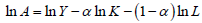, where

The growth rate is then generated, taking the first difference of lnA and then averaging over the period. We will designate the annual growth rate of TFP by TFPGR.

2.2. Foreign Direct Investment (FDI)

FDI is the main explanatory variable of our model. Data on FDI come from WDI. We use the share of net FDI flows as a percentage of GDP. Since we focus on the technology transfers that FDI can provide for host countries, we think it is more relevant to consider net values rather than gross values. More precisely, we use the average value of FDI, defined as a percentage of GDP, for our study period.

2.3. Natural Resource Rents (RENT)

This is a very important explanatory variable for our study. The variable “RENT” is taken from the World Bank Adjusted Saving Project database. This database is used in the empirical works on natural resource exploitation [20] . It has the advantage of consolidating separate rents of several mining products, country by country. Indeed, as noted by Rosser [21] , most studies on the natural resource curse focus on the specific behaviors associated with agents in the presence of rents generated by the exploitation of natural resources and not on economic dependence or on the distortion of the export structure related to the presence of natural resources. Therefore, it appears that a measure in terms of rent income from natural resources is most appropriate.

The computation of the values of this variable is done in several stages. In a first step, we obtain the unit rent by the difference between the price on the world market and the unit cost of extraction. For negative values of the unit rent, it is assumed that the result is due to incomplete data on extraction costs [22] . For these cases, an adjustment is made. It consists of taking the average of the most recent five-year positive unit rent for the country. In a second step, the unit rent is multiplied by the quantity extracted from the product under consideration; this operation leads to the desired rent. It should be noted that for our case, all natural resources are considered by summing up the rents obtained by product, and the final rent is then reported to the country’s GDP.

2.4. The Control Variables

2.4.1. The Initial Level of Total Factor Productivity (TFPinit)

Econometric growth regressions, in cross-sections, usually include the initial level of GDP as an explanatory variable to control the convergence effects. Although there is no clear theoretical basis for TFP convergence across countries, recent studies have suggested convergence towards a common technological frontier. Ayhan Kose, Prasad [23] highlighted this convergence in their paper on the effects of financial liberalization on productivity growth. In our case, we use the initial level of total factor productivity at the beginning of our period, particularly in 1995. We therefore expect a negative effect of the initial TFP level on TFP growth. It should be noted that our initial TFP will be expressed in logarithms in our econometric regressions.

2.4.2. The Credit Rate to the Private Sector (CREDIT)

This indicator considers loans granted to firms and households by banking and non-banking institutions (loans from the Central Bank to commercial banks and credits granted to the government and public enterprises are excluded), in relation to GDP. We chose it as an indicator of the size of financial development. It has been extracted from the WDI. In the literature on the determinants of TFP and economic growth, financial development plays an important role. King and Levine [24] show that financial development is of great importance for long-term productivity growth, as it makes it easier for entrepreneurs to finance their innovative projects. Aghion, Howitt [25] show that financial development is a key variable in explaining why some countries converge on the technological frontier while others diverge. Alfaro, Chanda [17] also show that the level of financial development of the host country plays an important role in determining the effect of FDI. In this paper, the financial development variable is designated by CREDIT and is expressed as a logarithm in the regressions. We expect a positive effect of this variable on TFP growth.

2.4.3. The Inflation Rate (INFLATION)

This is the consumer price index also extracted from the WDI. We consider it as an indicator of the macroeconomic environment, which is one of the main determinants of total factor productivity growth. Macroeconomic stability tends to stimulate long-term productivity growth, reduce interest rates and encourage entrepreneurs to spread their projects over a longer horizon. Aghion, Angeletos [26] have shown that this last aspect is particularly true in countries with low levels of financial development. We therefore control for the variable INFLATION, which is expressed as a logarithm in our regressions. A negative effect of inflation on TFP growth is naturally expected.

2.4.4. The Trade Openness (TRADE)

Trade liberalization also plays an important role in the literature on the determinants of TFP growth (see for example [27] ). We use as a measure of trade openness the share of imports and exports in GDP, as defined in the WDI from which the data are extracted. Trade openness can contribute to accelerating TFP by promoting the competitiveness of domestic producers and accelerating the integration of countries into the global economy. Increased competition between firms encourages innovations. The expected effect of trade openness―also expressed as a logarithm in our regressions―on the TFP growth is positive.

2.4.5. The Annual Growth Rate of the Population (POPGR)

POPGR is the annual growth rate of the population calculated over our study period. Data on population growth rate are extracted from the WDI. Population growth is one of the main variables found to be robust in growth regressions in the economic literature. Ayhan Kose, Prasad [23] controlled for it in their paper on the role of financial liberalization in the growth of TFP. Alfaro, Chanda [17] also introduced it in their study on the effect of FDI on economic growth. There is a divergence of viewpoints according to the role of population growth in economic or TFP growth. Some authors note that population growth reduces natural resources and per capita capital for many years. Other authors insist that a larger population can positively affect productivity. We therefore control for this variable to see its effect on the growth of TFP.

2.5. Descriptive Statistics

After the presentation of the main variables used in our study, we give in this section an overview of their descriptive statistics (Table 1). It can be noted that both the annual TFP growth rate and FDI (as a percentage of GDP) and the natural resource rent show significant variation in the database. The average value of the TFP growth rate is 0.97 percent, but it ranges from −4.67 percent to 4.79 percent. FDI also shows a great dispersion.

Table 2 shows the correlations between these key variables. In this respect, we can observe the negative correlation between the TFP growth rate and the natural resources rent. Similarly, although FDI is positively correlated with the TFP growth rate, the value of the correlation coefficient is not too important.

3. Empirical Strategy

3.1. The Model

Our study attempts to show the net effect of FDI on the TFP growth, considering the rent provided by natural resources and controlling for several variables. In the logic of Mankiw, Romer [28] , since there is a strong chance that countries are not in their regular state, we are also interested in the transitional dynamics that should be more important. Therefore, our dependent variable is the growth rate of TFP, instead of its level. To begin, we look at the direct effect of FDI on TFP growth by estimating the model with the Ordinary Least Squares (OLS) method. Our sample includes 71 developing countries. OLS method is applied to

the following equation:

(1)

We will focus on the estimated coefficients of the Equation (1) and more particularly on the coefficients in front of the FDI and RENT variables (β₂ and β₃, respectively). We check the consistency of the signs of the coefficients of our control variables with what we expected and presented in the presentation of the variables. Second, and this is also the key point of our study, we interact the variable FDI with the variable RENT and use it as an explanatory variable to capture the role of natural resources in determining the effect of FDI on TFP growth. The two variables FDI and RENT are still controlled in the equation, which is specified as follows:

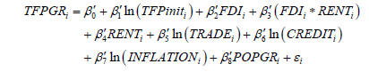(2)

In the specification of Equation (2), we will focus on the coefficients in front of the variables FDI and FDI*RENT.

3.2. The Issues of Endogeneity

An important issue in the relationship between FDI and TFP growth is the endogeneity of the FDI variable. Indeed, while FDI can broadly be a source of technology transfer and economic growth, it is also plausible that FDI itself will be determined to a large extent by the TFP growth. More specifically, a country with higher productivity growth may attract more FDI than a country with relatively smaller TFP growth. It is expected that a country with high-growth TFP will be more efficient in terms of adoption of new technologies and innovations, and this can be a fundamental determinant of foreign investors’ decisions regarding location. This is a specific case of a simultaneity bias that can be a source of endogeneity of the FDI variable. In addition, there may be an omission bias caused by the omission of a relevant variable correlated with FDI, as well as by errors in FDI measurement.

To solve this endogeneity problem, we will use an instrumental variable estimation method of two-stage least squares (IV). The instrumental variables must meet two conditions to be valid: they must be effectively correlated to the endogenous variable, and they must have no direct influence on the dependent variable (TFP growth). We will test the validity and non-weakness of our instruments and the endogeneity of the FDI variable in the following section. Here, we are just posing the problem.

We use three variables as instruments of the FDI variable: the country’s isolation (LANDLOCK), the lagged FDI (FDILAG) and the real exchange rate (EXR). Our variable LANDLOCK is a dummy variable that takes the value 1 if the country is landlocked and 0 if not. We think that the fact that a country is landlocked or not can affect the investment choice of foreign entrepreneurs especially because of the difficulties that can appear in the routing of imported products in the case of a landlocked country. Regarding the instrumental variable FDILAG, which represents the previous FDI (for the period 1985-1990), we drew on the economic literature. Wheeler and Mody [29] note that the current or existing stock of FDI is an important determinant of the successive foreign investments. In addition, Alfaro, Chanda [17] and Borensztein, De Gregorio [30] used lagged FDI as an instrumental variable in their studies.

Our third instrument―the real exchange rate (EXR)―is an important determinant of FDI among many others. Real exchange rates, by modifying the relative costs (or relative wealth), can have an impact on the investment decisions of multinational firms. For example, Froot and Stein [31] linked foreign investment decisions to the real exchange rate movements in a model of capital markets imperfection. In their model, a depreciation of the local currency, which also causes a depreciation of the real exchange rate, increases the relative wealth of foreign firms, which encourages them to invest abroad. Klein and Rosengren [32] also showed evidence of the real exchange rate as a significant determinant of FDI. The EXR variable is calculated in this paper as the ratio of domestic price relative to USD converted to the local currency. There is no reason to think that the EXR of a country can have a direct impact on a country’s TFP growth.

Finally, it should be noted that since the FDI variable is suspected of endogeneity, the introduction of any interactive variable involving FDI makes this new variable endogenous. This is the case of FDI*RENT in our Equation (2), which is our equation of interest. For this reason, we will also instrument this interactive variable, which to some extent represents the FDI in the natural resource sector generating rents in the corresponding countries. This interactive variable will be instrumented by FDILAG*RENT and LANDLOCK*RENT.

3.3. The Econometric Tests

3.3.1. The Test of Normality of Residuals

The normality test applied to our equation of interest gives us a statistic of 3.12 and a probability of committing a first-order error of 0.21². In other words, if we reject the null hypothesis of normality, there is a 21 percent chance of making a wrong decision. Since this probability is higher than the usual tolerance thresholds (1%, 5% or 10%), the hypothesis of normality of residuals is not rejected.

3.3.2. The Homoscedasticity Test

The White test applied to the equation of interest gives us a White statistic of 42.26 with a p-value of 0.50. The hypothesis of homoscedasticity is therefore not rejected at the usual tolerance thresholds, as the probability of committing an error by rejecting the null hypothesis is 50 percent. Correction of heteroscedasticity is therefore unnecessary³.

3.3.3. The Test of Non-Weakness of the Instruments

In the section on endogeneity issues, we underlined the likely endogeneity of the FDI and FDI*RENT variables. Thus, it appears necessary to apply the orthogonality test to confirm or refute our suspicion. However, one must make sure of the non-weakness of the instruments used. Using weak instrument variables to realize the orthogonality test makes this test less powerful, as the orthogonality hypothesis is often accepted wrongly. The test of non-weakness of instruments consists in checking whether the instruments are sufficiently correlated with the endogenous variables or whether the explanatory power of the instrumentation equations is quite important. As already highlighted above, the variables LANDLOCK, FDILAG and EXR are used as instruments of the FDI variable, and for the interactive variable FDI*RENT, the instrumental variables are LANDLOCK*RENT and FDILAG*RENT. When there are two or more endogenous variables, the instruments of each endogenous variable also instrument the other endogenous variables. We thus have two instrumentation equations, one for FDI and the other for FDI*RENT, in which the endogenous variables are regressed on the exogenous explanatory variables and on their five instruments, without omitting the constant. To ensure the non-weakness of the instruments, we test the joint significance of these instruments in the two equations with an F-test and calculate the partial R² (representing the explanatory power of the instruments).

We approximate the partial R² by the difference between the R² of the instrumentation equation and the R² of the same equation omitting the instrumental variables. Thus, for the FDI instrumentation equation, the joint significance test of the instruments gives us a Fisher statistic of 11.10 (p-value of 4.28 × 10⁻⁷), and the partial R² is 0.38. For FDI*RENT, we get a Fisher statistic of 67.19 (p-value of 2.98 × 10⁻¹⁰) and a partial R² of 0.55. These indicators show that the explanatory power of the instruments is important; they cannot be considered as weak⁴.

3.3.4. The Orthogonality Test

The aim is to test whether our suspected endogenous variables are endogenous or not, particularly the FDI and FDI*RENT. The orthogonality test used is that of Durbin, Wu and Hausman in the version of Nakamura and Nakamura [33] . In the null hypothesis of the orthogonality, the OLS estimator is convergent, with minimal variance. In the alternative hypothesis, the MCO estimator is non-convergent, while the two-stage least squares estimator (IV) is convergent.

The principle of the test is to remove the residuals of our two instrumentation equations estimated by the OLS and to introduce them as explanatory variables in our equation of interest. We obtain the test equation, and the objective will be to check whether the two residual variables are significant or not. In the latter case, we do not reject the null hypothesis of orthogonality of the variables suspected of endogeneity.

Applying this test, we get a Fisher statistic of 13.80 for a p-value of 1.84 × 10⁻⁵. We therefore reject the null hypothesis of orthogonality of the FDI and FDI*RENT variables and confirm the endogeneity of FDI and FDI*RENT. The two-stage least squares method will be applied to estimate our Equation (2)⁵.

3.3.5. The Over-Identification Test

This is a test to ensure the quality of instrumental variables [34] . It is only relevant when the number of instrumental variables is greater than the number of endogenous explanatory variables, which is true in our case (we have five instruments for two endogenous variables). The objective is to check the orthogonality of the instrumental variables with respect to the random errors. To do this, we estimate the test equation using OLS. The test equation is the regression of the residuals of Equation (2) (estimated by IV) on the five instruments and the other exogenous explanatory variables, without the constant. In the null hypothesis of the validity of the instruments, Sargan’s S statistic follows χ² whose degree of freedom is equal to the difference between the number of instruments (exogenous explanatory variables included) and the number of explanatory variables. In our case, S = NR² follows a χ² with 3 degrees of freedom. The statistic S is 1.062 with a p-value of 0.78. For the usual tolerance thresholds, we cannot reject the null hypothesis of the validity of the instruments⁶.

4. The Results and Discussion

Table 3 summarizes the main results of our econometric model. To begin, we examine the direct effect of FDI on the TFP growth. Remember that the idea is to see whether, based on our sample, FDI has any influence on TFP growth. The results of this first estimate by OLS, which appear in the first column of Table 3, confirm to some extent our conception about the effect of FDI on TFP growth. Indeed, the coefficient in front of FDI, although positive, is not significant; this may give a rough representation of the problem in the economic literature: while there is a strong theoretical basis for the positive effect of the FDI on productivity growth, the empirical evidence is still fragile. The FDI may have positive effects in some cases and negative effects in other cases. Therefore, there is no reason to believe that this effect will be positive or negative. This ambiguity of the FDI effect on TFP growth has motivated this paper regarding the role of natural resources in the relationship between FDI and TFP growth.

Let us now give an overview on the control variables of Equation (1). We can already note that the coefficient in front of TFP init (in logarithm) is negative and highly significant, which confirms the hypothesis of convergence. Indeed, it is likely that the higher the initial level of productivity, the lower the TFP growth will be. The natural resource rent variable has a significantly negative effect on the TFP growth. This result seems to validate the phenomenon of the natural resource curse. The financial development (CREDIT) also has a significant and positive effect on TFP growth, as expected. Inflation rate has a significantly

***, **,* significant at 1, 5, and 10 percent respectively; student t values in parentheses.

negative effect on the TFP growth, as macroeconomic instability may discourage investment and innovation. Population growth has a significant negative impact on productivity growth. Finally, although the coefficient of trade openness is positive as expected, it is not significant.

After this overview of our control variables, we turn to the results of the OLS estimation of Equation (2), in which we introduced an interactive variable FDI*RENT. The results are reported in the second column of Table 3. The estimated coefficient of FDI is positive and significant at 5 percent. The interactive variable FDI*RENT has a highly negative and significant effect on TFP growth. These results imply that the effect of FDI on TFP growth is positive but decreases with the natural resource rents. In other words, the net effect of FDI on TFP growth differs across countries, based on the availability of natural resources providing rents to the host countries. This result is of great importance, as it seems to be consistent with the theory of the natural resource curse. We will later try to give an explanation for this result. For now, let us observe the behavior of the other explanatory variables. The coefficient of the RENT variable, which was significantly negative in Equation (1), is no longer significant even if it is still negative. The introduction of the interactive variable FDI*RENT may have captured most of the effect of RENT variable. All the other control variables behave similarly as previously except the TRADE variable, whose coefficient is now negative but still insignificant.

We previously suspected (and confirmed our suspicions using the orthogonality test) the FDI and FDI*RENT variables of endogeneity. It is therefore necessary to estimate our Equation (2) using the two-stage least squares method, as the OLS method may substantively bias our results. The results are reported in the last column of Table 3. The explanatory power of the model is 0.25, which is not negligible since 25 percent of the TFP growth variability are explained by the model. The coefficient of FDI is still positive and significant at 10 percent, while the interactive variable is significantly negative at 10 percent. These results confirm what we previously found: the effect of FDI on TFP growth decreases with natural resource rents. However, it can be noticed that the coefficients are higher in absolute value, compared with those of the OLS. This can be explained, among other things, by the correction of an attenuation bias due to a conventional measurement error on the FDI. It may also be noted that the TRADE variable, representing the effect of trade openness, has a negative and significant (at 10 percent) effect on TFP growth; this result, which was not expected, can be explained by the import content of trade openness, which contributes to the decline in total factor productivity. Indeed, if imports consist mainly of food products and not capital and technology-intensive goods, the effect will not be favorable to the growth of TFP.

It would be interesting to have an estimate of the important role that natural resource rent can play in determining the net effect of FDI on TFP growth. For this purpose, we calculate the effect of a one standard deviation increase of the RENT variable on the TFP growth for a country receiving the average level of FDI in our sample. The effect is measured by β”₃*mean(IDE)*σ (RENT). It appears that a one standard deviation increase in natural resource rent reduces the FDI effect on TFP growth by 0.000062 percent.

One can also determine the level of RENT from which the net effect of FDI on TFP growth becomes negative, as this effect decreases with the natural resource rent. We derive our dependent variable (the TFP growth) relative to the FDI variable, and we equalize it to zero. We find a value of 21.78. This result just means that in our sample, if natural resources in a country generate an income above 21.78 percent of GDP, then the FDI has a negative net impact on TFP growth.

The effect of the FDI on TFP growth, which decreases with natural resource rents, can be explained by the combination of two factors. On the one hand, natural resources are themselves an important determinant of FDI, which means that FDI that goes to resource-rich countries is more oriented towards the natural resource sector. On the other hand, FDI in the sector of natural resources does not generate the expected benefits in terms of technology diffusion that can contribute to the growth of TFP. In fact, local companies can only benefit from the technology of multinational firms established in the country if they are either complementary or in competition. In the natural resources sector in many developing countries, this is not the case, and technology and skills transfers are often not effective.

5. Concluding Remarks

One of the fundamental reasons for the observed growth in foreign direct investment flows and the interest that countries, especially developing ones, have in receiving this FDI is the idea that FDI can contribute immensely to the development efforts of the host country. In fact, the FDI can be a source of technology transfer, strengthening the workforce through managerial skills and other externalities that benefit the host economies by increasing the total factor productivity. With the rise in these FDI flows, especially in developing countries, the natural question that may come to the mind of policymakers is whether an economy grows faster through FDI. The empirical literature, at both macroeconomic and microeconomic scales, has not found convincing evidence in favor of FDI.

The benefits of foreign investment may depend on local conditions in the host country. Based on a sample of 71 developing countries, we have attempted to show that the availability of natural resources in the countries and more precisely the rents that these natural resources provide can be an important determinant of the net effect of FDI on the growth of TFP. We empirically found that the effect of FDI on the TFP growth decreases with the natural resource rent. Thus, the gains of FDI in terms of productivity growth are lower in more natural resource-rich countries, highlighting the phenomenon of the natural resource curse.

This result is highly important, especially for sub-Saharan African countries where extractive industries receive the bulk of FDI. To turn this curse into a “blessing”, it would be wise to examine the establishment of policies and institutions regulating the participation of multinationals in the extractive industries in a development-friendly way and to put in place some measures to encourage the industrialization and diversification of the developing economies based on the extraction of natural resources.

Acknowledgements

The authors would like to thank the anonymous referees and the editor of the journal for useful comments and suggestions on the original version of this article.

Cite this paper

Zidouemba, P.R. and Elitcha, K. (2018) Foreign Direct Investment and Total Factor Productivity: Is There Any Resource Curse? Modern Economy, 9, 463-483. https://doi.org/10.4236/me.2018.93031

References

Appendices

***, **,*: significant at 1, 5, and 10 percent respectively; in parentheses the values of the student t.

***, **, *: significant at 1, 5, and 10 percent respectively; in parentheses the values of the student t.

The statistic of Sargan S = N*R² = 0.018*59 = 1.062 and χ²(3) = 7.8147 for an error of the first kind of 5 per cent, hence the non-rejection of the null hypothesis of the validity of the instruments.

NOTES

¹See the list of the countries included in this study in Table A1 of Appendices.

²Results not reported in this manuscript.

³We will correct, however, for the sake of efficiency gains. See Table A2 in Appendices for details of the test.

⁴See Table A3 in Appendices for the details of the test.

⁵The details of the test are presented in Table A4 in Appendices.

⁶Table A5 in Appendices for the presentation of the test results.

References

- 1. World Bank (2017) World Development Indicators (WDI). http://data.worldbank.org/data-catalog/world-development-indicators
- 2. Klenow, P.J. and Rodríguez-Clare, A. (2005) Chapter 11 Externalities and Growth. Handbook of Economic Growth, 1, 817-861. https://doi.org/10.1016/S1574-0684(05)01011-7
- 3. Easterly, W. and Levine, R. (2002) It’s Not Factor Accumulation: Stylized Facts and Growth Models. Central Banking, Analysis, and Economic Policies Book Series, 6, 61-114.
- 4. Wong, W.-K. (2007) Economic Growth: A Channel Decomposition Exercise. The BE Journal of Macroeconomics, 7, 1-38. https://doi.org/10.2202/1935-1690.1464
- 5. Lawer, E.T., Lukas, M.C. and Jørgensen, S.H. (2017) The Neglected Role of Local Institutions in the “Resource Curse” Debate. Limestone Mining in the Krobo Region of Ghana. Resources Policy, 54, 43-52. https://doi.org/10.1016/j.resourpol.2017.08.005
- 6. Siakwah, P. (2017) Are Natural Resource Windfalls a Blessing or a Curse in Democratic Settings? Globalised Assemblages and the Problematic Impacts of Oil on Ghana’s Development. Resources Policy, 52, 122-133. https://doi.org/10.1016/j.resourpol.2017.02.008
- 7. Harrison, A. and Rodríguez-Clare, A. (2010) Trade, Foreign Investment, and Industrial Policy for Developing Countries. In: Rodrik, D. and Rosenzweig, M.R., Eds., Handbook of Development Economics, Elsevier, Amsterdam, 4039-4214. https://doi.org/10.1016/B978-0-444-52944-2.00001-X
- 8. Haddad, M. and Harrison, A. (1993) Are There Positive Spillovers from Direct Foreign Investment? Journal of Development Economics, 42, 51-74. https://doi.org/10.1016/0304-3878(93)90072-U
- 9. Aitken, B., Harrison, A. and Lipsey, R.E. (1996) Wages and Foreign Ownership a Comparative Study of Mexico, Venezuela, and the United States. Journal of International Economics, 40, 345-371. https://doi.org/10.1016/0022-1996(95)01410-1
- 10. Aitken, B.J. and Harrison, A.E. (1999) Do Domestic Firms Benefit from Direct Foreign Investment? Evidence from Venezuela. American Economic Review, 89, 605-618. https://doi.org/10.1257/aer.89.3.605
- 11. Aturupane, C., Djankov, S. and Hoekman, B. (1999) Horizontal and Vertical Intra-Industry Trade between Eastern Europe and the European Union. Weltwirtschaftliches Archiv, 135, 62-81. https://doi.org/10.1007/BF02708159
- 12. Kinoshita, Y. (2001) R&D and Technology Spillovers via FDI: Innovation and Absorptive Capacity. University of Michigan Business School Working Paper, 349a.
- 13. Branstetter, L. (2006) Is Foreign Direct Investment a Channel of Knowledge Spillovers? Evidence from Japan’s FDI in the United States. Journal of International Economics, 68, 325-344. https://doi.org/10.1016/j.jinteco.2005.06.006
- 14. Carkovic, M. and Levine, R. (2005) Does Foreign Direct Investment Accelerate Economic Growth, in Institute for International Economics. Working Paper, University of Minnesota Department of Finance.
- 15. Balasubramanyam, V.N., Salisu, M. and Sapsford, D. (1996) Foreign Direct Investment and Growth in EP and Is Countries. The Economic Journal, 106, 92-105. https://doi.org/10.2307/2234933
- 16. Xu, B. (2000) Multinational Enterprises, Technology Diffusion, and Host Country Productivity Growth. Journal of Development Economics, 62, 477-493. https://doi.org/10.1016/S0304-3878(00)00093-6
- 17. Alfaro, L., et al. (2004) FDI and Economic Growth: The Role of Local Financial Markets. Journal of International Economics, 64, 89-112. https://doi.org/10.1016/S0022-1996(03)00081-3
- 18. Woo, J. (2009) Productivity Growth and Technological Diffusion through Foreign Direct Investment. Economic Inquiry, 47, 226-248. https://doi.org/10.1111/j.1465-7295.2008.00166.x
- 19. Wang, M. and Wong, M.C.S. (2009) Foreign Direct Investment and Economic Growth: The Growth Accounting Perspective. Economic Inquiry, 47, 701-710. https://doi.org/10.1111/j.1465-7295.2008.00133.x
- 20. Collier, P. and Hoeffler, A. (2005) Resource Rents, Governance, and Conflict. Journal of Conflict Resolution, 49, 625-633. https://doi.org/10.1177/0022002705277551
- 21. Rosser, A. (2010) The Political Economy of the Resource Curse: A Literature Survey. NBER Working Paper No. 15836.
- 22. Bolt, K., Matete, M. and Clemens, M. (2002) Manual for Calculating Adjusted Net Savings. Environment Department, World Bank, 1-23.
- 23. Ayhan Kose, M., Prasad, E.S. and Terrones, M.E. (2009) Does Openness to International Financial Flows Raise Productivity Growth? Journal of International Money and Finance, 28, 554-580. https://doi.org/10.1016/j.jimonfin.2009.01.005
- 24. King, R.G. and Levine, R. (1993) Finance and Growth: Schumpeter Might Be Right. The Quarterly Journal of Economics, 108, 717-737. https://doi.org/10.2307/2118406
- 25. Aghion, P., Howitt, P. and Mayer-Foulkes, D. (2005) The Effect of Financial Development on Convergence: Theory and Evidence. The Quarterly Journal of Economics, 120, 173-222.
- 26. Aghion, P., et al. (2010) Volatility and Growth: Credit Constraints and the Composition of Investment. Journal of Monetary Economics, 57, 246-265. https://doi.org/10.1016/j.jmoneco.2010.02.005
- 27. Alcalá, F. and Ciccone, A. (2004) Trade and Productivity. The Quarterly Journal of Economics, 119, 613-646. https://doi.org/10.1162/0033553041382139
- 28. Mankiw, N.G., Romer, D. and Weil, D.N. (1992) A Contribution to the Empirics of Economic Growth. The Quarterly Journal of Economics, 107, 407-437. https://doi.org/10.2307/2118477
- 29. Wheeler, D. and Mody, A. (1992) International Investment Location Decisions. Journal of International Economics, 33, 57-76. https://doi.org/10.1016/0022-1996(92)90050-T
- 30. Borensztein, E., De Gregorio, J. and Lee, J.W. (1998) How Does Foreign Direct Investment Affect Economic Growth? Journal of International Economics, 45, 115-135. https://doi.org/10.1016/S0022-1996(97)00033-0
- 31. Froot, K.A. and Stein, J.C. (1991) Exchange Rates and Foreign Direct Investment: An Imperfect Capital Markets Approach. The Quarterly Journal of Economics, 106, 1191-1217. https://doi.org/10.2307/2937961
- 32. Klein, M. and Rosengren, E. (1994) The Real Exchange Rate and Foreign Direct Investment in the United States: Relative Wealth vs. Relative Wage Effects. Journal of International Economics, 36, 373-389. https://doi.org/10.1016/0022-1996(94)90009-4
- 33. Nakamura, A. and Nakamura, M. (1981) On the Relationships among Several Specification Error Tests Presented by Durbin, Wu, and Hausman. Econometrica, 49, 1583-1588. https://doi.org/10.2307/1911420
- 34. Sargan, J.D. (1988) Contributions to Econometrics. Vol. 1, Cambridge University Press, Cambridge.
Appendices
Table A1. List of countries.
Table A2. Homoscedasticity test.
Table A3. Test of non-weakness instruments.