Received 1 July 2014; revised 1 August 2014; accepted 1 September 2014

ABSTRACT

This paper offer an artificial neural network (ANN) model to calculate drag force on an axisymmetric underwater vehicle by obtaining dataset from a computational fluid dynamic analysis. First, great effort was done to calculate the pressure and viscous data forces by increasing the precision and numerical data in order to extend and raise quality of dataset. In this step, numerous different geometry models (configurations of axisymmetric body) were designed, examined and evaluated input parameters including: diameter of body, diameter of nose disc, length of body, length of nose and velocity whereas outputs contain pressure and viscous forces. This dataset was used to train the ANN model. Feed-forward neural network (FFNN) is selected which is more common and suitable in this field’s study. A three-layer neural network was opted and after training this network, the results showed good agreement with CFD data. This study shows that applying the ANN model helps to reach final purpose in the least time and error, in addition a variety of tests can be performed to have a desired design in this way.

Keywords:

Drag Force, Feed-Forward Neural Networks, Back-Propagation Algorithm, AUV

1. Introduction

Several ways exist to measure drag force where nearly all of them are expensive and need time consuming, so it is necessary to find cheaper and faster ways to calculate forces. For designing an underwater body, obtaining operating forces on it is very important. Applications of computational methods to the maritime industry continue to grow as this advanced technology takes advantages of high speed computers. In the last two decades, different areas of incompressible flow modeling including grid generation techniques, solution algorithms and turbulence modeling, and computer hardware capabilities have witnessed tremendous development. In view of these developments, computational fluid dynamics can offer a cost-effective solution to many problems in underwater vehicle hull forms. However, effective utilization of CFD for marine hydrodynamics is also very expensive while a new approach which is called artificial neural network suggests a fast and cheap method to utilize preceding advantages.

To reduce drag force over underwater body, many researchers have worked and various approaches were created. Carmichael 1966 [1] used a method for torpedo-type shape in laminar flow. That study was to reduce drag force significantly by merely manipulating shape and a formal shape-synthesizing was developed. A method for the automatic synthesis of minimum drag hull on the axisymmetric vehicles in constant speed was determined by Parsons et al. 1974 [2] . Drag reduction was solely performed through the manipulation of hull shape. In their paper, eight classes of parameters related to the rounded-nose and tail boom bodies were taken into account to reach a well-behaved drag reduction. The results of lengthy analysis completely were explained by those eight parameters. The drag model was based on classical hydrodynamics and included the computer programs work available in literature. Sometimes the spatial formula for drag is useful such as formula appraised by the Freudenthal 2002 [3] . In order to compute the drag coefficient, a mean velocity with assumptions of a self similar wake and power low implementation from the wake scale on an axisymmetric body is used. To predict drag force on a prototype model of axisymmetric submarine hull in the water, tunnel experiments were carried out by him and then experimental results were compared to the CFD results. The new methods which are functions of shape, speed and size to estimate drag force were recommended by Paster et al. 2003 [4] and also this research was illustrated minimum correspond in volume where a reasonable hydrodynamic design could be resulted in little drag and noise. Estimating of drag force on the basis of the standard DREA¹ bare submarine hull was performed by Baker 2004 [5] .

In recent years, usage of ANN has been considered in many different fields in the maritime applications, for example the usage of ANN to find coefficients of state equations for an underwater vehicle’s motion in a horizontal plan and also researching about effect of neuron’s activation function on underwater vehicle’s motion quality by Zak 2005 [6] . Parameters of the underwater vehicle’s dynamics were identified by repeating optimization network. He also described operating principle of network and simulation result of underwater vehicle’s motion along a desired path and inserted quantity of state variables by a differential nonlinear model and a generated neural model.

Also another application of this technique is in autonomous underwater vehicle’s (AUV) depth control system in which there is uncertain nonlinear dynamic with unknown nonlinearities (Shi et al. 2007) [7] . Theses unknown nonlinearities are approached by the FFNN type of networks and their parameters were modified accommodative online in concord for a set of estimated laws variables for driving the AUV through cruise at the certain depth.

By using finite volume method based on Reynolds-Averaged Navier-Stokes (RANS) equations, Mashud Karim et al. 2008 [8] obtained viscous drag force. Computations were implemented on submarine bare hull DREA and six axisymmetric bodies for the Length-Diameter (L/D) ratios ranging from 4 to 10. They also used Shear Stress Transport (SST) k- model to simulate fully turbulence flow past bodies.

The important component of the drag is the wave resistance related to sea surface deformation because of the wave motion of platform. The reason of usage of a torpedo-like shape by Alvares et al. 2009 [9] is the optimum hull shape of underwater vehicle that moved near the sea surface. They worked on the underwater vehicles (AUVs) where have been built traditionally autonomous. In this case, In this case, they also considered using the first-order Rankine panel method to compute the wave resistance for the body. They measured the total drag of the scaled models in torpedo shape for determine results of the optimum shapes.

The study of different profiles to achieve proper geometry in head portion through computational analysis could help to understand the hydrodynamics of underwater body as Suman et al. 2010 [10] appraised functionality of an ellipsoidal head and concocted hydrodynamic performance which improved at a high speed for underwater vehicle. They understood that ellipsoidal nose profile could improve the cavitation vulnerability better and also minimize the overall drag of the vehicle.

In present study it has been tried to estimate pressure and viscous drag force on the axisymmetric body (see Figure 1) using a code which is produced with neural network.

Multilayer perceptron was selected because this type was suitable for this investigation and Feed-forward network typically trained with static back-propagation algorithm. First, many numerical data were obtained then trained the network and results illustrated as graphs that show good agreement with the data impounded for network phase test. With this approach one code has obtained that could predict forces in many configurations and supply net data of drag forces with given varying conditions.

2. Governing Equation

The governing equations for the mathematical description of fluid flow are written in the Eulerian framework. The averaged transport equation for conservation of mass may be written as:

(1)

where ρ is the mass density and u is the fluid velocity vector.

The averaged momentum equation for fluid is:

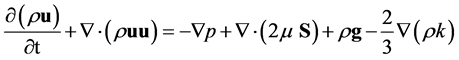(2)

where ρ is the pressure of the gas phase, g is the gravitational acceleration, is the effective viscosity of the gas, k is the turbulence kinetic energy, and S is the symmetric part of the velocity gradient tensor.

For the closure of the above equations, the transport equations for turbulence kinetic energy and its dissipation have to be solved.

3. Artificial Neural Network

From the style of the human brain, ANN is constructed by Hakeem [11] and has been widely used in fields such as pattern recognition, optimization, and coding, financial, industrial, medic by Cacciola et al. 2010 [12] , metallurgy by Chehreh Chelgani et al. 2010 [13] , chemical by Hoskins et al. 1988 [14] and Bhat et al. 1989 [15] , etc. which had given exactness and competence whereas has specific ability to solve bulky and stubborn problems form learning a specific way from given data. In nature, ANN could be given a set of outputs with given set of inputs data by constructing some mapping relationships by Afkhami et al. 2008 [16] . It has a high degree of pliability which could easily be taken the nonlinearly behavior by the processing data.

The training of the network model is done with using the Levenberg-Marquardt approach by Hagan et al. 1994 [17] and 1996 [18] . FFNN in engineering applications certainly are most common neural network fashion. The three-layer of FFNN could depict sufficient number of neurons from any functions whereas previous provided by Cybenko et al. 1989 [19] . FFNN normally included three layers: input layer, hidden layer and an output layer thus is related to problem where hidden layer can be increased. The FFNN where have been used for this investigation are shown in Figure 2. The role of input layer is getting the inputs data and transmit them to hidden layer that each of the neurons from hidden layer do two tasks: 1) all of the inputs multiplied by weights numbers and 2) these data pass a transfer function with nonlinear modification manner, then the outputs of the neurons in hidden layer becomes inputs data for the neurons of the output layer.

Finally the output layer do some procedures similar to hidden layer with own neurons and give the numerical data as outputs result from FFNN. In former phase transfer functions such as hyperbolic tangent, sigmoid, linear algebra, etc. could be selected for each of the hidden and output layers in sake of their applications.

In this problem sigmoid is selected as transfer function that is very common in these cases. The FFNN with N neurons in the input layer is specified by and N weights showed by , whereas input term could be determined like the following:

(3)

The input of the each hidden layer will be some which will transmit from a sigmoid function showed below and they are converted as a data for the other step.

(4)

And this style is repeated for entire data through all layers till the epochs were finished or network reached to threshold. Training from data is the spirit of neurons computing. Each processing element has versatile parameters which must be changed in agreement with some prespecified procedures that back-propagation algorithm is the most common form of learning rules then the weights are changed to correspond with their prior value and a correction term. Momentum was selected as the learning rule with step size one. Maximum epoch’s iteration was prepared whereas how much iteration should be done to satisfied the criterion. The errors get from difference the desired (targets) and the value predicted by network (output) and has several ways to compute such as normalized mean squared error (NMSE), mean absolute error (MAE), mean squared error (MSE), minimum squared error and minimum absolute error. The conventional measuring and the most popular for fitting data is MSE. The MSE for computing error was used by following equation

(5)

where P is number of output processing elements, N is number of exemplars in the data set, is network output for exemplar i at processing element j and is desired output exemplar i at processing element j. Now in this paper to estimate pressure and viscous drag forces, a network has been designed with eight processing elements in the one hidden layer with sigmoid function as a transfer function and used of five inputs such as velocity, diameter and length of body, length of nose and diameter of nose that are illustrated in the Figure 2.

After training the ANN model, the ability of the networks for predicting unseen data has to be checked. For this purpose, several patterns for all ranges are generated to test the ANN model. With applying the neural network and setting the details of ANN structure, a close range of data should be provided where it helps to get nearly exact outputs of network and then select the optimal structure by choice learning algorithm’s type, the number of hidden layer, etc.

If the dimensional of an axisymmetric underwater body has wanted to be specified, problem could be solved as a reverse problem that the inputs for introducing network became pressure and viscous drag forces which will give the dimensions of ideal body.

4. Result and Discussion

Used algorithm is like quasi-Newton methods and approaching to the second order training speed without computation of Hassian matrix. Here the Hassian matrix would be approximated as:

(6)

and gradient could be computed as follows:

(7)

where J is Jacobin matrix includes the first derivatives of the networks error with respect to the weights, and e is a vector of networks errors.

(8)

where is a positive scalar and I is a unit matrix. If is large, then the algorithm became gradient descent with a small step size. This algorithm did not make any improvement either in the training time or in the degree of generalization obtained. Sometimes it becomes snarled in local minim which was too far from the absolute one although using the information related to the second derivate of the error (deflexion of the surface) to reach the minimum value. If error is combined from numerous crests and troughs, the algorithm will care for converge in the nearest trough, which might be a local minimum. Otherwise if the error were simpler and primary weight vector was located in the vicinity of the absolute minimum, it would be expected to be converged faster than most of the training methods.

The results of the networks for weights and biases are shown in the Tables 1-3. Using these values some algebraic expression can adjust that will give the pressure and viscous drag forces easily and fast.

In all figures the ANN model could capture those styles almost well. The mean error, variance, and algebraic expression between desired and output of network model are shown in Table 4.

In present study, 577 training patterns are generated by using CFD analysis and were used as inputs to predict the output parameters. The most becoming attire for the ANN model was obtained with attempt on several network models that were created, trained, and tested. Errors computed for even smaller change in the details of ANN model such as number of layers, the transfer function, the hidden layers, etc. for integrated layers and

segregated layers with the proper criterion coefficients that had worthwhile of utilizing time. The multilayer perception as is integrated with FFNN model, the back-propagation algorithm (BP), and the momentum learning rule which applied to adjust the weights for the input and output layers. Errors by BP algorithm computed and went to backward layers that for each epoch it has been tried to reduce errors in successive layer until satisfied the criterion coefficient. The 5-8-2 (number of neurons in each layer) ANN model was found in a way that it could predict the pressure and viscous drag forces with different conditions. The numerical data computed by CFD analysis are shown in Figure 3 as the static pressure with respect to changes in position.

In the Figure 4, the contour of static pressure is shown for upper half of underwater body and it can be seen that the maximum static pressure is in the first point of contact i.e. stagnation point and the velocity is zero, consequently pressure became maximum and almost over the nose arc, body is monotonous and over the tail it becomes additive with former reason.

All of the data need to be normalized before introducing network model and the network by this manipulation could predict better. First a set of 15 samples of total dataset was separated for testing network model and it was started to train one by one by samples, and the process of reducing error that computed by MSE was continued and used to adjust the weights in each epoch using BP algorithm and momentum rule for leaning as an iterative supervised technique, till the MSE reaches to 0.000106, it means the network model attained a good mood to predict desired data as it is shown in Figure 5.

The set of testing data which applied to see how good the model is after working on all details of networks model, showed that the present model could estimate the pressure and viscous drag forces satisfactorily. The data were obtained by the ANN model are in good agreement with the unseen data for network. The behavior of ANN model versus desired data in Figure 6 is illustrated and shows this agreement between both of dataset (desired and output), and it means that the ANN model follows the desired data which is the scope of this study.

The pressure and viscous drag forces for four values of velocity are illustrated in Figure 7 and it can be seen that predicted values are nearly close to the desired data. In these figures it is evident that by increasing the velocity, the pressure force decreases on the basis of Euler equation and this phenomenon can be easy proved using differential equation. Viscous drag force, Reynolds number and velocity behave the same way by increasing

the velocity and are increased, consequently viscous force decreases.

As it was seen for the length of body parameter in Figure 8, pressure drag force increases reasonably by raising the length. Here the state of viscous force is similar to the prior case which increasing the length of body Reynolds number led to an increase and therefore this force decreased consequently. For diameter of nose disc parameter that is shown in Figure 9, until the value of 0.6, decrease in the pressure force can be seen which is caused by increasing diameter of nose disc in the Euler equation, the height of water on the body became low and therefore the differential pressure decreases too.

Differential pressure multiplied by area and the results decrease because of effect of declining differential pressure which is more than raise in value of area.

For value of 0.8, this routine changes and magnitude of area becomes more than the differential pressure and consequently the pressure force is increased that was seen one jump to bigger value.

About viscous drag force a reducing march until value of 0.6 can be seen in the figure. To explain this, the viscous force over the body, length of the nose arc, and tail of underwater body should be considered. In those sections, viscous force merely over the length of the nose arc is effective and also has a remarkable growth whereas the others has very little changes, then increasing the velocity to position ratio is the reason of increasing the viscous force and it’s important on the arc.

At value of 0.8 it can be seen a nearly constant viscous force over the nose arc than a high variation over the length of body that took a low value than prior and in this condition the streamline over body are smoother as velocity to position ratio had low value at 0.8 than the value of 0.6. In Figure 10, pressure drag force with increasing the diameter of body has a reducing progress. This case is similar to the pervious about increasing the diameter of nose disc as that reason was explained. Also viscous drag force versus diameter of body has a reducing progress that its reason is associated with Reynolds number. By increasing Reynolds number by augment the diameter (instead of length of body could have diameter in some cases), viscous drag force with pervious reason was reduced like to related velocity case.

In Figure 11 for length of nose arc which pressure drag force is increased by raising the length of nose arc. The pressure force over each section for this case has changed but merely on the nose arc increased a lot as it is also negative and the others had a very little change and the reason of increased pressure force over nose arc is increasing the length in area as pervious case about increasing the length of body and results between negative value of nose arc and positive values from the others is declined in the pressure force. Viscous force increased on both of shear stress from velocity to position ratio and length of nose arc increased and therefore viscous force increased too.

The usage of the ANN proved that it could give a simpler formula to obtain favorite data and have much practical applications and wonderful advantages. This technique could consume very little time with an acceptable error. Now instead of running one state for a few days and then decide about results, only with a few seconds it

is done and provides several states to select the best solution for related problem. Figure 12 shows vary and benefits of applying the ANN. This chart is only indicating time-used for doing one state by these two methods and in order to that is presented here showing significance of ANN results versus CFD results with consideration cost and time of course after provided needed data to operate in ANN manner. In CFD running, nearly 4 hours is required for only one state, while the ANN training with too sensitiveness about 10 minutes (surely related to quantity of data and settings) and one testing with usage of obtained equations from ANN merely one second or less was needed. To present more comparisons in this field several experiments will be done from other aspects and a few different CFD procedures with applying ANN that will be future works whereas would be bring more comparisons of precise and influences of cavitations, roughness, noise etc. The purpose of Figure 12 was only showing time-used that could be improved and desired time can be reached in next applications.

5. Conclusion

The FFNN process was applied to estimate the pressure and viscous drag forces. An FFNN with 5-8-2 neuron in input-hidden-output layer organization was found which could obtain the value of them with good accuracy and in the least time. This approach could be applied in the inverse way or extend more details from sections of axisymmetric underwater body for both drag forces and inputs data. To abtain more choices, this approach is really useful and practical whereas become independent of so many experiments and large coding to calculate prototype data. The ideal condition had more data until errors trend to zero. In all cases for pressure and viscous drag force, the big and the small error are about 3.75 and 0.54 respectively which could be satisfactory. With this weights and biases, some equations could be driven for estimating the pressure and viscous drag forces solely from dimensions and also could be used as a cost function in optimization algorithm. This research shows that we can economize in time considerably and extend the range of dataset for designing and also use this method in other works.

References

NOTES

¹Defence Research Establishment Atlantic.

References

- Carmichael, B.H. (1966) Underwater Vehicle Drag Reduction Through Choice of Shape. AIAA Paper 66-657.
- Parsons, J.S. and Goodsont, R.E. (1974) Shaping of Axisymmetric Bodies for Minimum Drag in Incompressible Flow. AIAA. Journal of Hydronautics, 8, NO. 3.
- Freudenthal, J.L. (2002) Experimental Studies on the Drag of an Axisymmetric Hull. Thesis in Aerospace Engineering, Mississippi.
- Paster, D., Raytheon, Co. and Portsmouth, R.I. (2003) Importance of Hydrodynamic Considerations for Underwater Vehicle Design. IEEE Oceans, 18, 1413-1422.
- Baker, C. (2004) Estimating Drag Force on Submarine Hulls. Report DRDC Atlantic CR2004-125, Defence R&D Canada-Atlantic.
- Zak, B. (2005) The Neural Model of Dynamics of Unmanned Underwater Vehicle. EUSFLAT-LFA Conference, Gdynia, 506-511.
- Shi, Y., Qian, W., Yan, W. and Li, J. (2007) Adaptive Depth Control for Autonomous Underwater Vehicles Based on Feed forward Neural Networks. International Journal of Computer Science & Applications, 4, 107-118.
- Karim Md., M., Rahman Md., M. and Alim Md., A. (2008) Numerical Computation of Viscous Drag for Axisymmetric Underwater Vehicles. Journal of Mechanical and Industrial Engineering, 9-21.
- Alvarez, A., Bertram, V. and Gualdesi, L. (2009) Hull Hydrodynamic Optimization of Autonomous Underwater Vehicles Operating at Snorkeling Depth. Ocean Engineering, 36, 105-112. http://dx.doi.org/10.1016/j.oceaneng.2008.08.006
- Suman, K.N.S., Rao, D.N., Das, H.N. and Kiran, G.B. (2010) Hydrodynamic Performance Evaluation of an Ellipsoidal Nose for a High Speed under Water Vehicle. Jordan Journal of Mechanical and Industrial Engineering, 4, 641-652.
- Hakeem, M.A., Kamil, M. and Arman, I. (2008) Prediction of Temperature Profiles Using Artificial Neural Networks in a Vertical Thermosiphon Reboiler. Applied Thermal Engineering, 28, 1572-1579.
- Cacciola, M., Megali, G., Fiasché, M., Versaci, M. and Morabito, F.C. (2010) A Comparison between Neural Networks and k-Nearest Neighbours for Blood Cells Taxonomy. Memetic Computing, 2, 237-246. http://dx.doi.org/10.1007/s12293-010-0043-6
- Chehreh Chelgani, S., Shahbazi, B. and Rezai, B. (2010) Estimation of Froth Flotation Recovery and Collision Probability Based on Operational Parameters Using an Artificial Neural Network. International Journal of Minerals, Metallurgy and Materials, 17, 526-534. http://dx.doi.org/10.1007/s12613-010-0353-1
- Hoskins, J.C. and Himmelblau, D.M. (1988) Artificial Neural Network Models of Knowledge Representation in Che- mical Engineering. Computers & Chemical Engineering, 12, 881-890. http://dx.doi.org/10.1016/0098-1354(88)87015-7
- Bhat, N. and McAvoy, T. (1989) Use of Neural Nets for Dynamic Modeling and Control of Chemical Process Systems. American Control Conference, Pittsburgh, 21-23 June 1989, 1336-1341.
- Afkhami, A., Abbasi-Tarighat, M. and Bahramb, M. (2008) Artificial Neural Networks for Determination of Enantiomeric Composition of α-Phenylglycine Using UV Spectra of Cyclodextrin Host-Guest Complexes: Comparison of Feed-Forward and Radial Basis Function Networks. Talanta, 75, 91-98.
- Hagan, M.T. and Menhaj, M. (1994) Training Feed-Forward Networks with the Marquardt Algorithm. IEEE Transactions on Neural Networks, 5, 989-993. http://dx.doi.org/10.1109/72.329697
- Hagan, M.T., Demuth, H.B. and Beale, M.H. (1996) Neural Network Design. PWS Publishing, Boston.
- Cybenko, G. (1989) Approximation by Superpositions of a Sigmoid Function. Mathematics of Control, Signals and Systems, 2, 303-314.
NOTES
1Defence Research Establishment Atlantic.