 Journal of Applied Mathematics and Physics, 2016, 4, 1592-1599 Published Online August 2016 in SciRes. http://www.scirp.org/journal/jamp http://dx.doi.org/10.4236/jamp.2016.48169 How to cite this paper: Osman, A. and Haji, A. (2016) Well-Posedness of an N-Unit Series System with Finite Number of Vacations. Journal of Applied Mathematics and Physics, 4, 1592-1599. http://dx.doi.org/10.4236/jamp.2016.48169 Well-Posedness of an N-Unit Series System with Finite Number of Vacations Abdugeni Osman, Abdukerim Haji College of Mathematics and Systems Science, Xinjiang University, Urumqi, China Received 12 May 2016; accepted 17 August 2016; published 24 August 2016 Abstract We investigate the solution of an N-unit series system with finite number of vacations. By using -semigroup theory of linear operators, we prove well-posedness and the existence of the unique positive dynamic solution of the system. Keywords N-Unit Series System, -Semigroup, Dynamic Solution, Well-Posedness 1. Introduction The study of repairable systems is an important topic in reliability. The series system is one of the classical re- pairable systems. Since the strong practical background of the series systems, many researchers have studied them extensively under varying assumptions on the failures and repairs, see [1]-[4]. In [4], the authors studied an N-unit series system with finite number of vacations and obtained some reliability expressions such as the Lap- lace transform of the reliability, the mean time to the first failure, the availability and the failure frequency of the system. In [4], the authors used the dynamic solution in calculating the availability and the reliability. But they did not discuss the existence of the positive dynamic solution. Motivated by this, we study in this paper the well-posedness and the existence of a unique positive dynamic solution of the system, by using -semigroup theory of linear operators. For background reading on semigroup theory we refer to [5] or [6]. The N-unit series system with finite number of vacations can be described by the following equations (see [4]). ( R ) + Λ 0 ( ) = ( ) 0 ( , ) +∞ 0 , + + ( ) ( , ) =0,=1,2,,, + + ( ) ( , ) = 0 ( , ) ,=1,2,,,=1,2,,, + + Λ+ ( ) 0 ( , ) =0,=1,2,,, 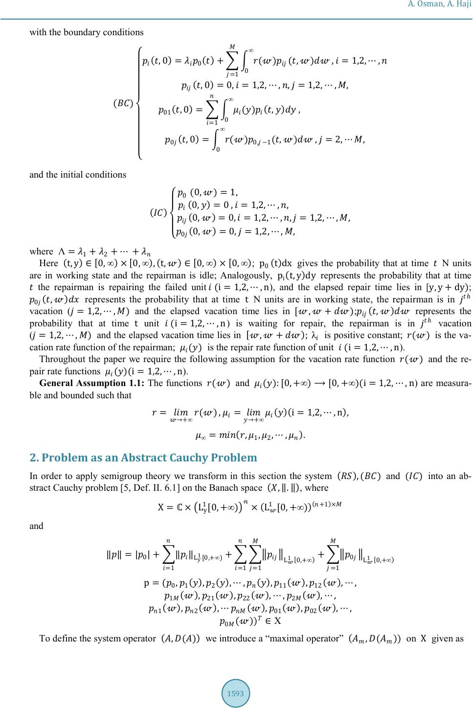 A. Osman, A. Haji with the boundary conditions ( ) ( ,0 ) = 0 ( ) + () (,) ∞ 0 =1 ,=1,2,, ( ,0 ) =0,=1,2,,,=1,2,,, 01 ( ,0 ) = () ( , ) ∞ 0 , =1 0 ( ,0 ) =() 0,1 (,) ∞ 0 ,=2,, and the initial conditions ( ) 0 ( 0, ) =1, ( 0, ) =0 ,=1,2,,, ( 0, ) =0,=1,2,,,=1,2,,, 0 ( 0, ) =0,=1,2,,, where Λ= 1 + 2 + + Here ( t,y ) [ 0,∞ ) × [ 0,∞ ) , ( t, ) [ 0,∞ ) × [ 0,∞ ) ; p 0 ( t ) dx gives the probability that at time N units are in working state and the repairman is idle; Analogously, p i ( t,y ) dy represents the probability that at time the repairman is repairing the failed unit (i=1,2,,n), and the elapsed repair time lies in [y,y + dy); 0 ( , ) represents the probability that at time t N units are in working state, the repairman is in vacation (=1,2,,) and the elapsed vacation time lies in [,+ ); ( , ) represents the probability that at time t unit (i=1,2,,n) is waiting for repair, the repairman is in vacation (=1,2,,) and the elapsed vacation time lies in [ ,+ ) ; λ is positive constant; () is the va- cation rate function of the repairman; () is the repair rate function of unit (i=1,2,,n). Throughout the paper we require the following assumption for the vacation rate function () and the re- pair rate functions ()(i=1,2,,n). General Assumption 1.1: The functions () and ():[0,+∞)[0,+∞)(i=1,2,,n) are measura- ble and bounded such that = +∞ (), = +∞ ( )( i=1,2,,n ) , ∞ = ( , 1 , 2 ,, ) . 2. Problem as an Abstract Cauchy Problem In order to apply semigroup theory we transform in this section the system ( ) ,() and () into an ab- stract Cauchy problem [5, Def. II. 6.1] on the Banach space ( , . ) , where X=× L y 1 [0,+∞) × ( L 1 [0,+∞) ) ( +1 ) × and = | 0 | + L y 1 [0,+∞) + L 1 [ 0,+∞ ) =1 =1 + 0 L 1 [ 0,+∞ ) =1 =1 p=( 0 , 1 ( ) , 2 ( ) ,, ( ) , 11 ( ) , 12 ( ) ,, 1 ( ) , 21 ( ) , 22 ( ) ,, 2 ( ) ,, 1 ( ) , 2 ( ) , ( ) , 01 ( ) , 02 ( ) ,, 0 ( ) ) Χ To define the system operator ( ,() ) we introduce a “maximal operator” ( ,( ) ) on X given as 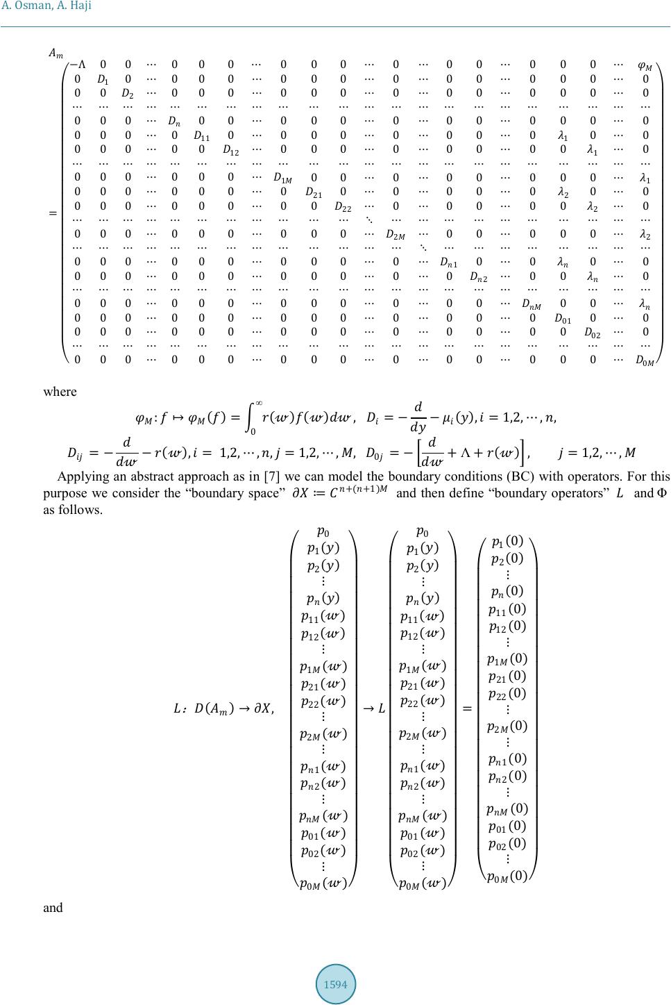 A. Osman, A. Haji = 00000000000000 0 1 00000000000000 00 2 0000000000000 000 000000000000 0000 11 00000000 1 00 00000 12 00000000 1 0 000000 1 00000000 1 0000000 21 00000 2 00 00000000 22 00000 2 0 000000000 2 00000 2 0000000000 1 00 00 00000000000 2 00 0 0 00000000000 00 0000000000000 01 00 00000000000000 02 0 000000000000000 0 where : ( ) = ( ) ( ) ∞ 0 , = ( ) ,=1,2,,, = ( ) ,= 1,2,,,=1,2,,, 0 = + Λ+ ( ) ,=1,2,, Applying an abstract approach as in [7] we can model the boundary conditions (BC) with operators. For this purpose we consider the “boundary space” +(+1) and then define “boundary operators” and Φ as follows. : ( ) , 0 1 ( ) 2 ( ) ( ) 11 ( ) 12 ( ) 1 () 21 () 22 () 2 () 1 () 2 () () 01 () 02 () 0 () 0 1 ( ) 2 ( ) ( ) 11 ( ) 12 () 1 () 21 () 22 () 2 () 1 () 2 () () 01 () 02 () 0 () = 1 ( 0 ) 2 ( 0 ) ( 0 ) 11 ( 0 ) 12 (0) 1 (0) 21 (0) 22 (0) 2 (0) 1 (0) 2 (0) (0) 01 (0) 02 (0) 0 (0) and 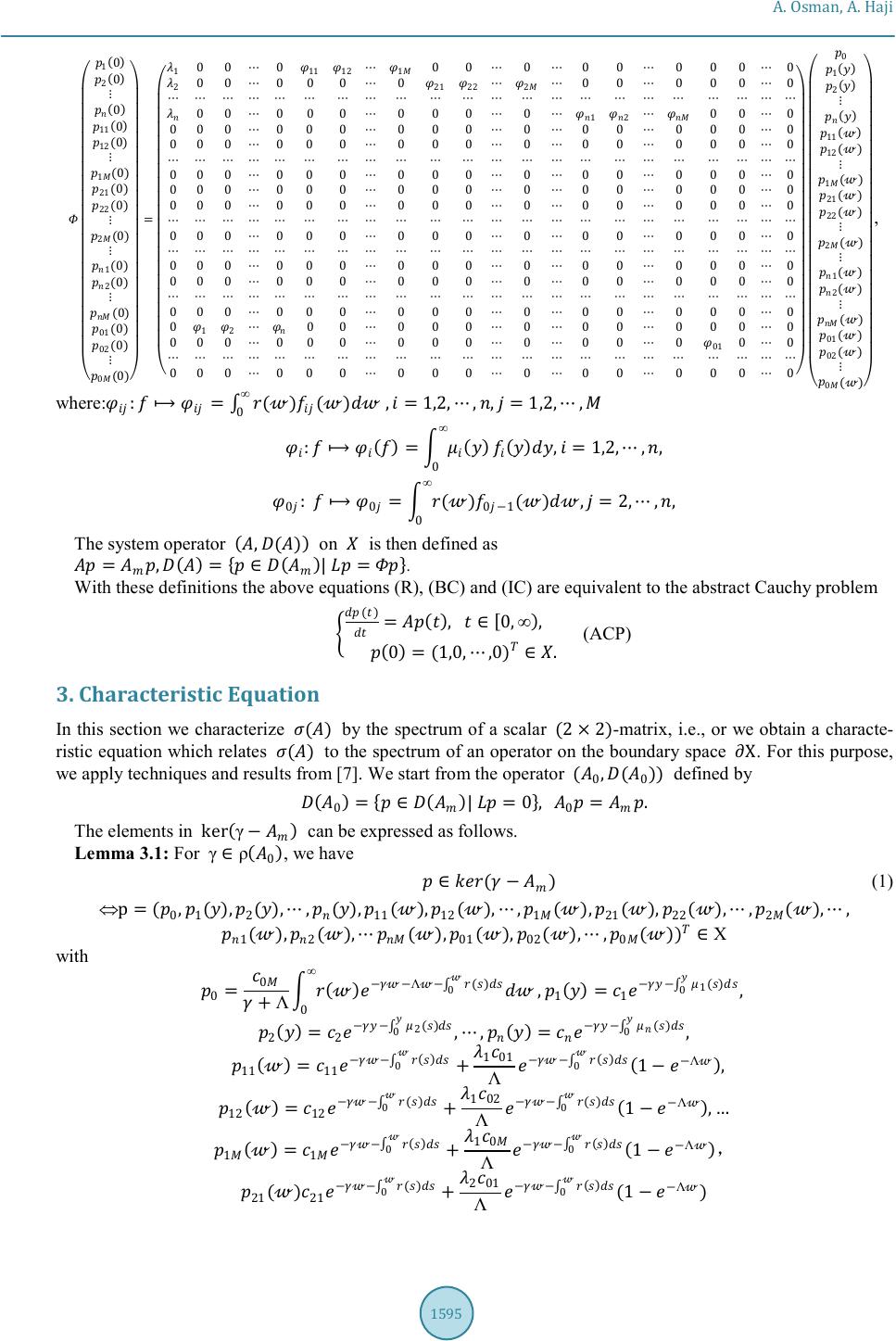 A. Osman, A. Haji 1 ( 0 ) 2 ( 0 ) ( 0 ) 11 ( 0 ) 12 (0) 1 (0) 21 (0) 22 (0) 2 (0) 1 (0) 2 (0) (0) 01 (0) 02 (0) 0 (0) = 1 000 11 12 1 000000000 2 000000 21 22 2 000000 000000000 1 2 000 0000000000000000 0000000000000000 0000000000000000 0000000000000000 0000000000000000 0000000000000000 0000000000000000 0000000000000000 0000000000000000 0 1 2 000000000000 0000000000000 01 00 0000000000000000 0 1 ( ) 2 ( ) ( ) 11 ( ) 12 () 1 () 21 () 22 () 2 () 1 () 2 () () 01 () 02 () 0 () , where: : = ( ) ( ) ,=1,2,,,=1,2,, ∞ 0 : ( ) = ( ) ∞ 0 ( ) ,=1,2,,, 0 : 0 = ( ) 01 ( ) ,=2,,, ∞ 0 The system operator ( ,() ) on is then defined as = , ( ) = { ( ) | = } . With these definitions the above equations (R), (BC) and (IC) are equivalent to the abstract Cauchy problem () = ( ) , [ 0,∞ ) , ( 0 ) =(1,0,,0) . (ACP) 3. Characteristic Equation In this section we characterize () by the spectrum of a scalar ( 2 × 2 ) -matrix, i.e., or we obtain a characte- ristic equation which relates () to the spectrum of an operator on the boundary space X. For this purpose, we apply techniques and results from [7]. We start from the operator ( 0 ,( 0 ) ) defined by ( 0 ) = { ( ) | =0 } , 0 = . The elements in ker ( γ ) can be expressed as follows. Lemma 3.1: For γρ ( 0 ) , we have ( ) (1) ⇔p=( 0 , 1 ( ) , 2 ( ) ,, ( ) , 11 ( ) , 12 ( ) ,, 1 ( ) , 21 ( ) , 22 ( ) ,, 2 ( ) ,, 1 ( ) , 2 ( ) , ( ) , 01 ( ) , 02 ( ) ,, 0 ( ) ) Χ with 0 = 0 + Λ ( ) Λ ( ) 0 ∞ 0 , 1 ( ) = 1 1 ( ) 0 , 2 ( ) = 2 2 () 0 ,, ( ) = ( ) 0 , 11 ( ) = 11 ( ) 0 + 1 01 Λ ( ) 0 ( 1 Λ ) , 12 ( ) = 12 () 0 + 1 02 Λ ( ) 0 ( 1 Λ ) ,… 1 ( ) = 1 ( ) 0 + 1 0 Λ ( ) 0 ( 1 Λ ) , 21 ( ) 21 () 0 + 2 01 Λ ( ) 0 ( 1 Λ ) 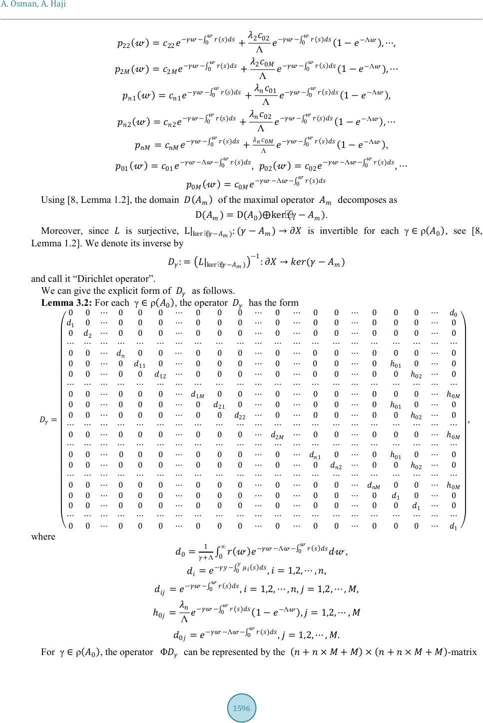 A. Osman, A. Haji 22 ( ) = 22 () 0 + 2 02 Λ ( ) 0 ( 1 Λ ) ,, 2 ( ) = 2 () 0 + 2 0 Λ ( ) 0 ( 1 Λ ) , 1 ( ) = 1 ( ) 0 + 01 Λ ( ) 0 ( 1 Λ ) , 2 ( ) = 2 () 0 + 02 Λ ( ) 0 ( 1 Λ ) , = () 0 + 0 Λ ( ) 0 ( 1 Λ ) , 01 ( ) = 01 Λ () 0 , 02 ( ) = 02 Λ () 0 , 0 ( ) = 0 Λ () 0 Using [8, Lemma 1.2], the domain ( ) of the maximal operator decomposes as D ( ) =D( 0 )ker(γ ). Moreover, since is surjective, L| ker ( ) :( ) is invertible for each γρ ( 0 ) , see [8, Lemma 1.2]. We denote its inverse by :=| ker ( ) 1 :( ) and call it “Dirichlet operator”. We can give the explicit form of as follows. Lemma 3.2: For each γρ ( 0 ) , the operator has the form = 00000000000000 0 1 00000000000000 0 2 0000000000000 00 000000000000 000 11 00000000 01 00 0000 12 00000000 02 0 00000 1 00000000 0 000000 21 00000 01 00 0000000 22 00000 02 0 00000000 2 00000 0 000000000 1 00 01 00 0000000000 2 00 02 0 00000000000 00 0 000000000000 1 00 0000000000000 1 0 00000000000000 1 , where 0 = 1 +Λ ( ) Λ ( ) 0 ∞ 0 , = ( ) 0 ,=1,2,,, = ( ) 0 ,=1,2,,,=1,2,,, 0 = Λ ( ) 0 ( 1 Λ ) ,=1,2,, 0 = Λ () 0 ,=1,2,,. For γρ ( 0 ) , the operator Φ can be represented by the ( + × + ) × ( + × + ) -matrix 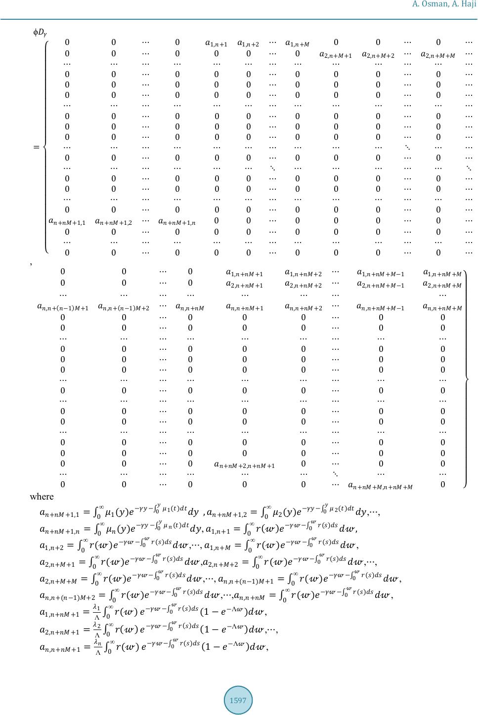 A. Osman, A. Haji ϕ = 000 1,+1 1,+2 1,+ 000 000000 2,++1 2,++2 2,++ 000000000 000000000 000000000 000000000 000000000 000000000 000000000 000000000 000000000 000000000 ++1,1 ++1,2 ++1, 000000 000000000 000000000 , 000 1,++1 1,++2 1,++1 1,++ 000 2,++1 2,++2 2,++1 2,++ ,+ ( 1 ) +1 ,+ ( 1 ) +2 ,+ ,++1 ,++2 ,++1 ,++ 0000000 0000000 0000000 0000000 0000000 0000000 0000000 0000000 0000000 0000000 000 ++2,++1 000 00000 ++,++ 0 where ++1,1 = 1 () 1 () 0 ∞ 0 , ++1,2 = 2 () 2 () 0 ∞ 0 ,, ++1, = () () 0 ∞ 0 , 1,+1 = ( ) ( ) 0 ∞ 0 , 1,+2 = () () 0 ∞ 0 ,, 1,+ = () () 0 ∞ 0 , 2,++1 = () () 0 ∞ 0 , 2,++2 = () () 0 ∞ 0 ,, 2,++ = () () 0 ∞ 0 ,, ,+(1)+1 = () () 0 ∞ 0 , ,+ ( 1 ) +2 = () () 0 ∞ 0 ,, ,+ = () () 0 ∞ 0 , 1,++1 = 1 Λ () ∞ 0 ( ) 0 ( 1 Λ ) , 2,++1 = 2 Λ ( ) ∞ 0 ( ) 0 ( 1 Λ ) ,, ,++1 = Λ () ∞ 0 ( ) 0 ( 1 Λ ) , 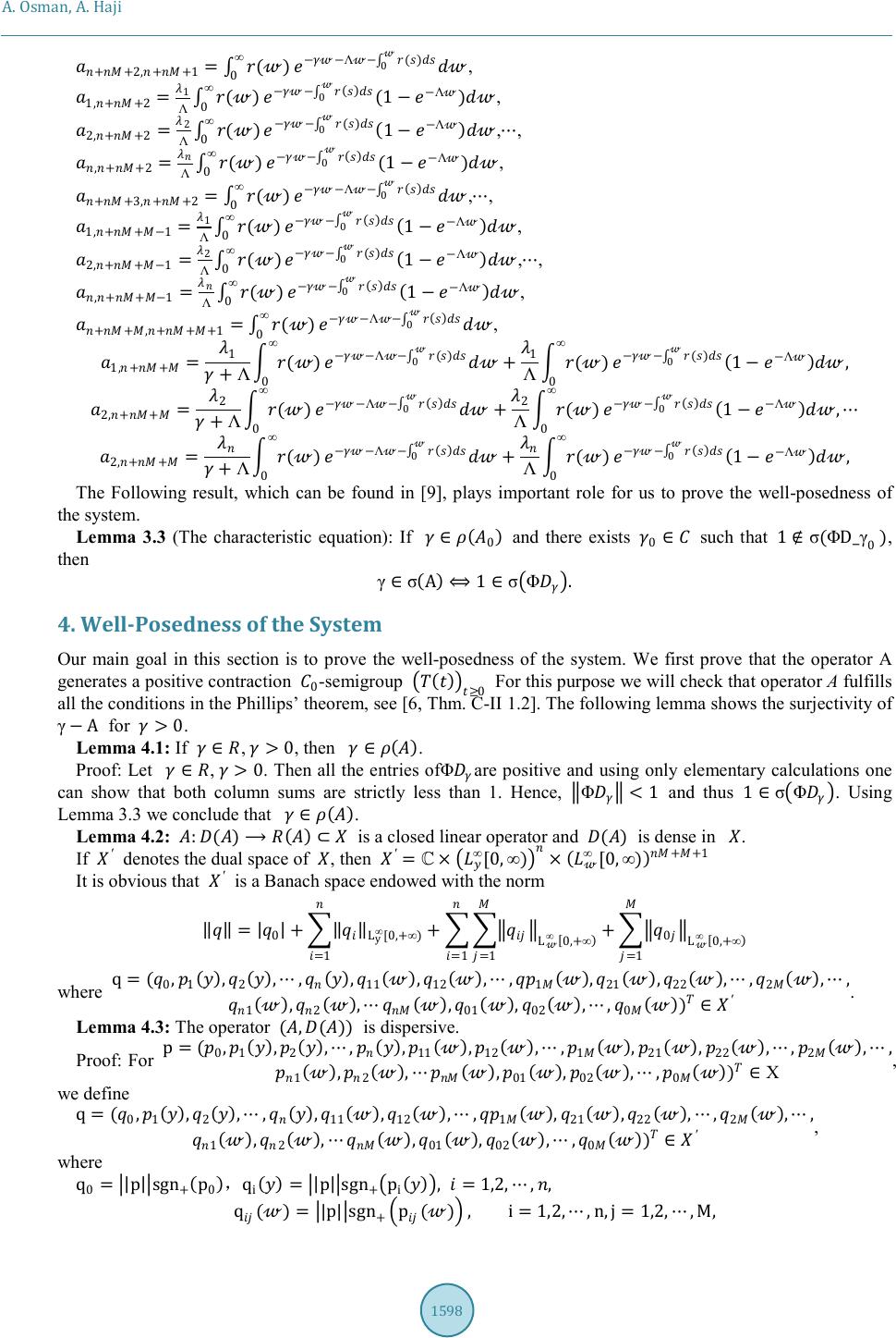 A. Osman, A. Haji ++2,++1 = () ∞ 0 Λ ( ) 0 , 1,++2 = 1 Λ () ∞ 0 ( ) 0 ( 1 Λ ) , 2,++2 = 2 Λ () ∞ 0 ( ) 0 ( 1 Λ ) ,, ,++2 = Λ () ∞ 0 ( ) 0 ( 1 Λ ) , ++3,++2 = () ∞ 0 Λ ( ) 0 ,, 1,++1 = 1 Λ () ∞ 0 ( ) 0 ( 1 Λ ) , 2,++1 = 2 Λ () ∞ 0 ( ) 0 ( 1 Λ ) ,, ,++1 = Λ () ∞ 0 ( ) 0 ( 1 Λ ) , ++,+++1 = () ∞ 0 Λ ( ) 0 , 1,++ = 1 + Λ () ∞ 0 Λ ( ) 0 + 1 Λ () ∞ 0 ( ) 0 ( 1 Λ ) , 2,++ = 2 + Λ () ∞ 0 Λ ( ) 0 + 2 Λ () ∞ 0 ( ) 0 ( 1 Λ ) , 2,++ = + Λ () ∞ 0 Λ ( ) 0 + Λ () ∞ 0 ( ) 0 ( 1 Λ ) , The Following result, which can be found in [9], plays important role for us to prove the well-posedness of the system. Lemma 3.3 (The characteristic equation): If ( 0 ) and there exists 0 such that 1σ(ΦD_γ 0 ), then γσ ( A ) 1σΦ . 4. Well-Posedness of the System Our main goal in this section is to prove the well-posedness of the system. We first prove that the operator A generates a positive contraction 0 -semigroup ( ) 0 For this purpose we will check that operator A fulfills all the conditions in the Phillips’ theorem, see [6, Thm. C-II 1.2]. The following lemma shows the surjectivity of γA for >0. Lemma 4.1: If , >0, then ( ) . Proof: Let , >0. Then all the entries ofΦ are positive and using only elementary calculations one can show that both column sums are strictly less than 1. Hence, Φ <1 and thus 1σΦ . Using Lemma 3.3 we conclude that ( ) . Lemma 4.2: :() ( ) is a closed linear operator and () is dense in . If ′ denotes the dual space of , then ′ =× ∞ [0,∞) × ( ∞ [0,∞) ) ++1 It is obvious that ′ is a Banach space endowed with the norm = | 0 | + L y ∞ [0,+∞) + L ∞ [ 0,+∞ ) =1 =1 + 0 L ∞ [ 0,+∞ ) =1 =1 where q=( 0 , 1 ( ) , 2 ( ) ,, ( ) , 11 ( ) , 12 ( ) ,, 1 ( ) , 21 ( ) , 22 ( ) ,, 2 ( ) ,, 1 ( ) , 2 ( ) , ( ) , 01 ( ) , 02 ( ) ,, 0 ( ) ) ′ . Lemma 4.3: The operator (,()) is dispersive. Proof: For p=( 0 , 1 ( ) , 2 ( ) ,, ( ) , 11 ( ) , 12 ( ) ,, 1 ( ) , 21 ( ) , 22 ( ) ,, 2 ( ) ,, 1 ( ) , 2 ( ) , ( ) , 01 ( ) , 02 ( ) ,, 0 ( ) ) Χ , we define q=( 0 , 1 ( ) , 2 ( ) ,, ( ) , 11 ( ) , 12 ( ) ,, 1 ( ) , 21 ( ) , 22 ( ) ,, 2 ( ) ,, 1 ( ) , 2 ( ) , ( ) , 01 ( ) , 02 ( ) ,, 0 ( ) ) ′ , where q 0 = | p | sgn + ( p 0 ) ,q i ( ) = | p | sgn + p i ( ) ,=1,2,,, q ( ) = | p | sgn + p ( ) ,i=1 ,2,,n,j=1,2,,M,  A. Osman, A. Haji q 0 ( ) = | p | sgn + p 0 ( ) ,j=1,2,,M, and sgn + ( p 0 ) = 1if p 0 >0, 0if p 0 0, sgn + p i ( y ) = 1if p i ( ) >0, 0if p i ( y ) 0, =1,2,,, sgn + p ( ) = 1if p ( ) >0, 0if p ( ) 0, i=1,2,,n,j=1,2,,M, sgn + p 0 ( ) = 1if p 0 ( ) >0, 0if p 0 ( ) 0, j=1,2,,M. Noting the boundary condition, it is not difficult to see that , 0. By [6, p.49] we obtain that ( ,() ) is a dispersive operator. From Lemma 4.1- 4.3 we see that all the conditions in Phillips' theorem (see [6, Thm. C-II 1.2]) are fulfilled and thus we obtain the following result. Theorem 4.4: The operator ( ,() ) generates a positive contraction 0 -semi-group ( ) 0 . From Theorem 4.4 and [5, Cor.II.6.9] we can characterize the well-posedness of The system ( ) , ( ) and ( ) as follows. Theorem 4.5: The system ( ) , ( ) and ( ) is well-posed. Combining Theorem 4.5 with [5, Prop.II.6.2] we can state our main result. Theorem 4.6: The system ( ) , ( ) and ( ) has a unique positive dynamic solution p(t)=( 0 (), 1 ( , ) , 2 ( , ) ,, ( , ) , 11 ( , ) , 12 ( , ) ,, 1 ( , ) , 21 ( , ) , 22 ( , ) ,, 2 ( , ) ,, 1 ( , ) , 2 ( , ) , ( , ) , 01 ( , ) , 02 ( , ) ,, 0 ( , ) ) Acknowledgements This work was supported by the National Natural Science Foundation of Xinjiang Uighur Autonomous Region (No. 2014211A002). References [1] Liu, R.B., Tang, Y.H. and Luo, C.Y. (2007) A New Kind of N-Unit Series Repairable System and Its Reliability Anal- ysis. Math. Appl, 20, 164-170. [2] Liu, R.B., Tang, Y.H. and Cao, B.S. (2008) A New Model for the N-Unitseries Repairable System and Its Reliability Analysis. Chinese Journal of Engineering Mathematics, 25, 421-428. [3] Kovalyov, M.Y., Portmann, M.C. and Oulamara, A. (2006) Optimaltesting and Repairing a Failed Series System. J. Comb. Optim, 12, 279-295. http://dx.doi.org/10.1007/s10878-006-9633-0 [4] Liu, R.B. and Liu, Z.M. (2011) Reliability Analysis of an N-Unit Series Repairable System with Finite Number of Va- cations. Operations Research and Management Science, 20, 102-107. [5] Engel, K.-J. and Nagel, R. (2000) One-Parameter Semigroups for Linear Evolution Equations. Graduate Texts in Ma- thematics, 194, Springer-Verlag. [6] Nagel, R. (1986) One-Parameter Semigroups of Positive Operators. Springer-Verlag. [7] Casarino, V., Engel, K.-J., Nagel, R. and Nickel, G. (2003) A Semigroup Approach to Boundary Feedback Systems. Integr. Equ. Oper. Theory, 47, 289-306. http://dx.doi.org/10.1007/s00020-002-1163-2 [8] Greiner, G. (1987) Perturbing the Boundary Conditions of a Generator. Houston J. Math., 13, 213-229. [9] Haji, A. and Radl, A. (2007) A Semigroup Approach to Queueing Systems. Semigroup Forum, 75, 610-624. http://dx.doi.org/10.1007/s00233-007-0726-6  Submit or recommend next manuscript to SCIRP and we will provide best service for you: Accepting pre-submission inquiries through Email, Facebook, LinkedIn, Twitter, etc. A wide selection of journals (inclusive of 9 subjects, more than 200 journals) Providing 24-hour high-quality service User-friendly online submission system Fair and swift peer-review system Efficient typesetting and proofreading procedure Display of the result of downloads and visits, as well as the number of cited articles Maximum dissemination of your research work Submit your manuscript at: http://papersubmission.scirp.org/
|