Journal of Electromagnetic Analysis and Applications
Vol.4 No.7(2012), Article ID:21269,7 pages DOI:10.4236/jemaa.2012.47043
Analysis of Land Subsidence Using the HES
![]()
Department of Intelligent Mechanical Engineering, Faculty of Engineering, Fukuoka Institute of Technology, Fukuoka, Japan.
Email: kswitsar@kmitl.ac.th, murayama@fit.ac.jp
Received May 2nd, 2012; revised June 4th, 2012; accepted June 16th, 2012
Keywords: HES; Incline; LSSM; Magnetic Field; Subsidence
ABSTRACT
This study presents a methodology for analysis of the industrial machine alignment in the production line. The level of land subsidence in the area of the industrial machine location was assessed by adopting Hall Effect Sensor (HES). A computer was used for real-time data collecting and displaying the angle of subsidence over operational period. The measurement module consists of two flat-curve permanent magnets mounted parallelly and the magnetic poles which were placed in position that can be generating the magnetic tension force. The center between two permanent magnets was the sensor namely HES placed perpendicularly to the magnetic fluxes. The permanent magnets were the moving parts which can be displaced depending on the inclined angle of land subsidence. Analysis of the relationship between the incline angle of the measurement module and the output voltage from the HES was considered from the function of subsidence angle and magnetic density on X-axis and perpendicular angle (Y-axis) with the resolution of 100 mV per degree. There were two ranges of measurement according to the angle resolution, –20 to 20 degree at 1 degree of resolution per step and –6 to 6 degree at 0.01 degree of resolution per step.
1. Introduction
Industrial production line is one of the most important processes as it is dependent on the quality of products from manufacturing process. Therefore, the machines used in this process should provide good performance. Appropriate machine alignment and also building construction should be prepared for preventing ground subsidence. However, the most common problem would be the error in machine operation caused by the level of land subsidence in the areas where a number of large and heavyload machines are placed. Generally, the angle can be measured by using several methodologies [1-4]. Angular measurement based on magnetic field method using the HES was the alternative methodology to measure and monitor land subsidence. The measured results were in electrical voltage form obtained from output of HES and then transmitted to computer for real time monitoring and maintaining the appropriate position of the machines.
2. Fundamental Method
2.1. Sensing Part and Error Analysis
HES is a small passive transducer (non-contact sensor) which is applicable in several purposes. The output voltage is generated when the constant current transmitting through a semiconductor namely Hall Generator is diverted [5,6]. In this study, the magnetic density (B) generated by sensing module can be analyzed by Lorenzt force (F) of the magnetic field on an electron (q) when changing the relative angle (q) and v is the velocity of electron due to electric field as given in Equation (1) [7].
 (1)
(1)
The output voltage from sensing of the HES (VH) as a function of the magnetic density can be calculated by Equations (2) and (3).
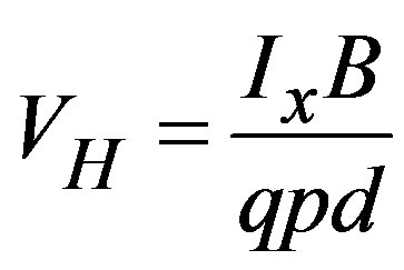 (2)
(2)
 (3)
(3)
where I is the current flowing through Hall generator on X-axis (A);
B is the density of magnetic field (Tesla);
d is the thickness of Hall generator (mm);
p is the number of holes;
n is the number of electrons.
The evaluation of value from repetitive measurements or random measurements is the estimation of uncertainty in type A standard. The standard deviation (Sd) will be considered as Estimate standard deviation in Equation (4) [8] when n is a great amount, x is the measured value.
 (4)
(4)
2.2. Principle of Permanent Magnet
The permanent magnet, ferromagnetic material type, was selected in this study and the maximum magnetic density was 0.25 Tesla. Two flat-curve permanent magnets was 10 mm wide, 1.5 mm thick, and 41.5 mm long. The outer and inner radius was 24 mm and 19 mm, respectively and the plate curve was 120 degree with the distance of 12 mm. The permanent magnet was mounted parallelly and the magnetic poles were placed in position that can generate the magnetic tension force and can provide the widest linearity range of magnetic density field as shown in Figures 1 and 2.
3. Structure of System Developed
The subsidence monitoring system presented in this study was developed by applying magnetic field method. There are three important parts of this system is as following; magnetic Field Generation, measuring system (Land subsidence sensing module) and electrical signal system. Details are as follows:
3.1. Magnetic Field Generation
To define the permanent magnet shape for generating the magnetic field, COMSOL software simulation was adopted. The permanent magnets were then positioned to generate magnetic flux in Y-axis direction. Two sets of four magnetic domains (one set consists two domains) were placed alternately in poles as shown in Figure 3. The appropriate gap of two permanent magnets was fixed at 12 mm, which was half the length of the outer radius of permanent magnet (24 mm). The result obtained from simulation is as shown in Figure 4 where Y-axis is the density of the magnetic field and X-axis is the inclination angle within the permanent magnet radius.
Figure 5 shows the direction of the flat-curve permanent magnet movement. The HES was placed at the center of magnets and perpendicular to X-axis. From experiment, the relationship between output voltage from the HES and magnetic field density generated by two flat-curve permanent magnets were observed. The results agree well to the results from calculation using COMSOL software simulation as shown in Figure 6 [9]. It can be noted that when the permanent magnet was moved, the output voltage from HES would be significantly varied
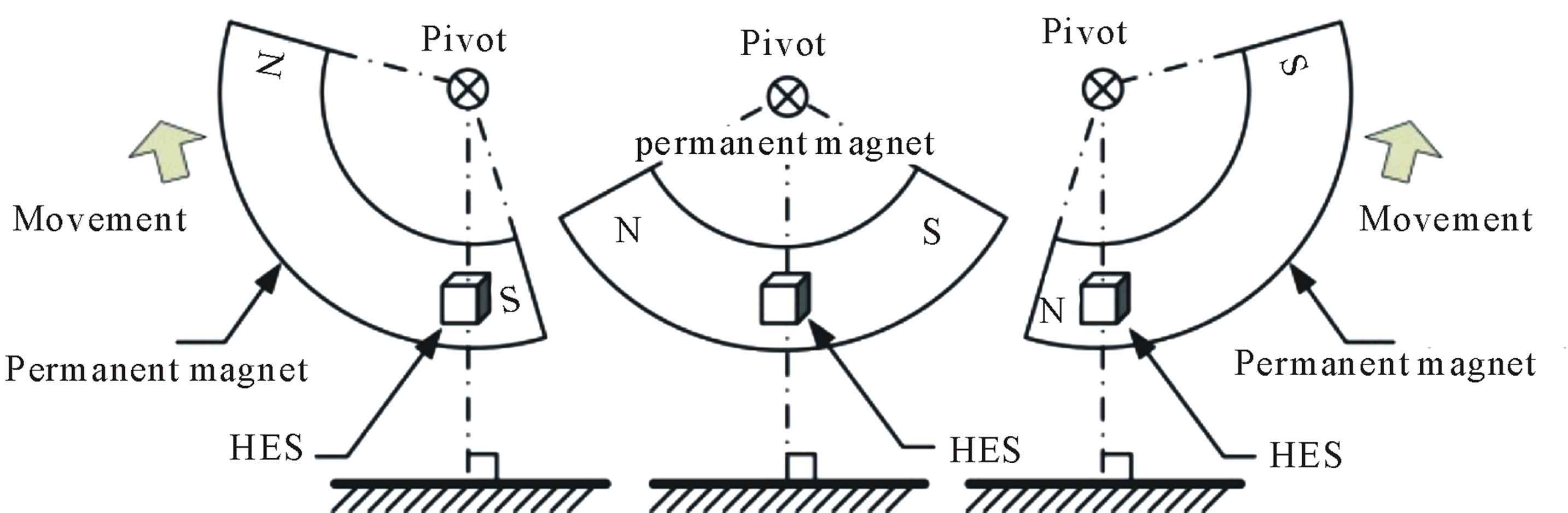
Figure 1. Direction of flat-curve permanent magnet movement.
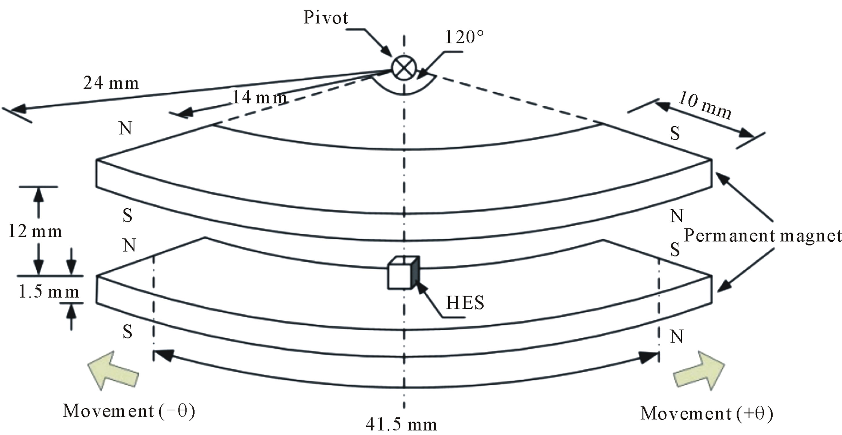
Figure 2. Structure of permanent magnetic and HES placement.
Figure 3. Characteristic of the magnetic flux was analyzed from the permanent magnet placed alternately in the poles by using COMSOL software simulation.
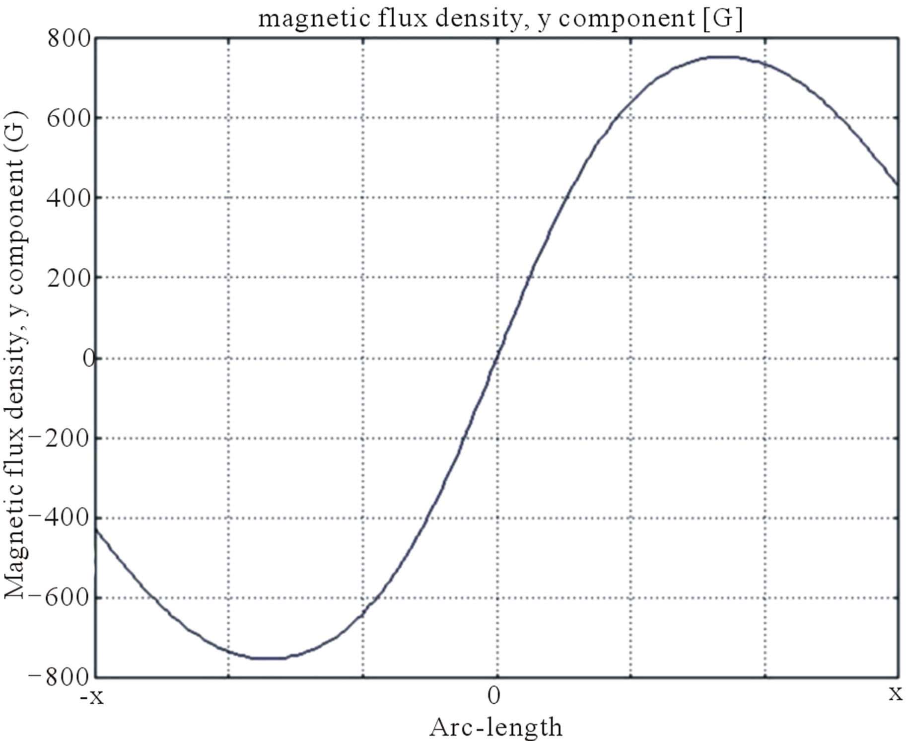
Figure 4. Wave form of magnetic field using COMSOL software.
at the middle range of permanent magnet. Moreover, it can provide the widest measuring range compared to other different magnet shapes. Therefore, the flat-curve permanent magnet was selected as in this study.
3.2. Land Subsidence Sensing Module
Profile of the measuring system namely Land subsidence sensing module (LSSM) consists of a sensor namely HES [10], placed at the center between two flat-curve permanent magnetic plates with the distance of 12 mm.
At the set point of 0 degree as shown in Figure 7.

Figure 5. Measured range of flat-curve permanent magnet.

Figure 6. Wave form of output voltage and magnetic field from experiment.
From experiment, the Land Subsidence Sensing Module (LSSM) exhibited high accuracy and reliability. The output voltage from inclination of angle experimented was calibrated using high accurate and precious instruments to setup the system developed as shown in Figures 8 and 9.
Figure 9 illustrates the angle calibration due to magnetic field movement. The high accurate and precious instrument (reference scale) for inclined angle adjustment was installed and defines the position of set point at 0 degree.

Figure 7. Profile of the LSSM at set point position (0 degree).

Figure 8. System alignment.

Figure 9. Angle calibration and reference angle measurement.
3.3. Electrical Signal System
The electrical signal system was developed by considering the voltage output of HES which is related to the magnetic density. The variation of output voltage is a function of the displacement of permanent magnets moving away from the center on X-axis that causes the distortion of magnetic fields interacting with HES. Therefore, the output voltage was varied by the density and direction of magnetic field. This voltage was compared to the constant reference signal (5 V) provided to the circuit by IC # Ref02 and then converted to digital signal by 24-bit ADC before transferring to microcontroller (AT89S52) for processing. Digital signal was finally transmitted to computer for collecting and analyzing data at a specified time interval by using database program developed. Block diagram of the system in overall is as shown in Figure 10.
4. Monitoring System
The inclined angel was examined using the LSSM based on magnetic field. Monitoring and displaying modules has been design and developed to show the results of the measurement of land subsidence. The measured results were in electrical voltage form obtained from output of HES. Data were sent to a computer for analyzing and processing through LabVIEW software as shown in Figure 11.
There were two ranges of analysis according to the angle resolution: 0.01 degree of resolution per step (the

Figure 10. Block diagram of overall system.
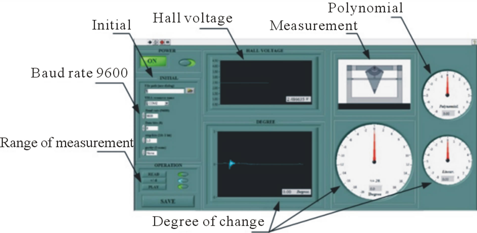
Figure 11. Subsidence monitoring system.
highest resolution) as shown in Figure 12 and 1 degree per step as shown in Figure 13. From Figure 13, the system developed can alert on the monitor in case of the inclined angles over range by more than 20 degree.
5. Experimental Observation
The system developed was designed to be inclined on X-axis in both (+) and (–) directions ranging from –40 to 40 degree. The measured results were agreed well to the results from calculation as shown in Figure 14. The results can also be expressed by the variation of output voltage through a third degree polynomial as given Equation (5) and the regression value is provided in Equation (6). Considering the output voltage variation from HES and magnetic field density when the LSSM displacing and tilting away from floor level, it was found that the maximum variation of output voltage from HES with the linearity and high accuracy was in the ranges of –20 to 20 degree. However, the relationship of output voltage and inclined angle can provide the best linearity and the most accuracy of the results in the range of –6 to 6 degree. Therefore, the experiments would be divided into two ranges: –20 to 20 degree and –6 to 6 degree.
y = –3E – 05x3 + 0.004x2 – 0.0788x + 1.3774(5)
R² = 0.9889 (6)
where y is output voltage from the HES (volt);
x is ranges of measurement (degree);
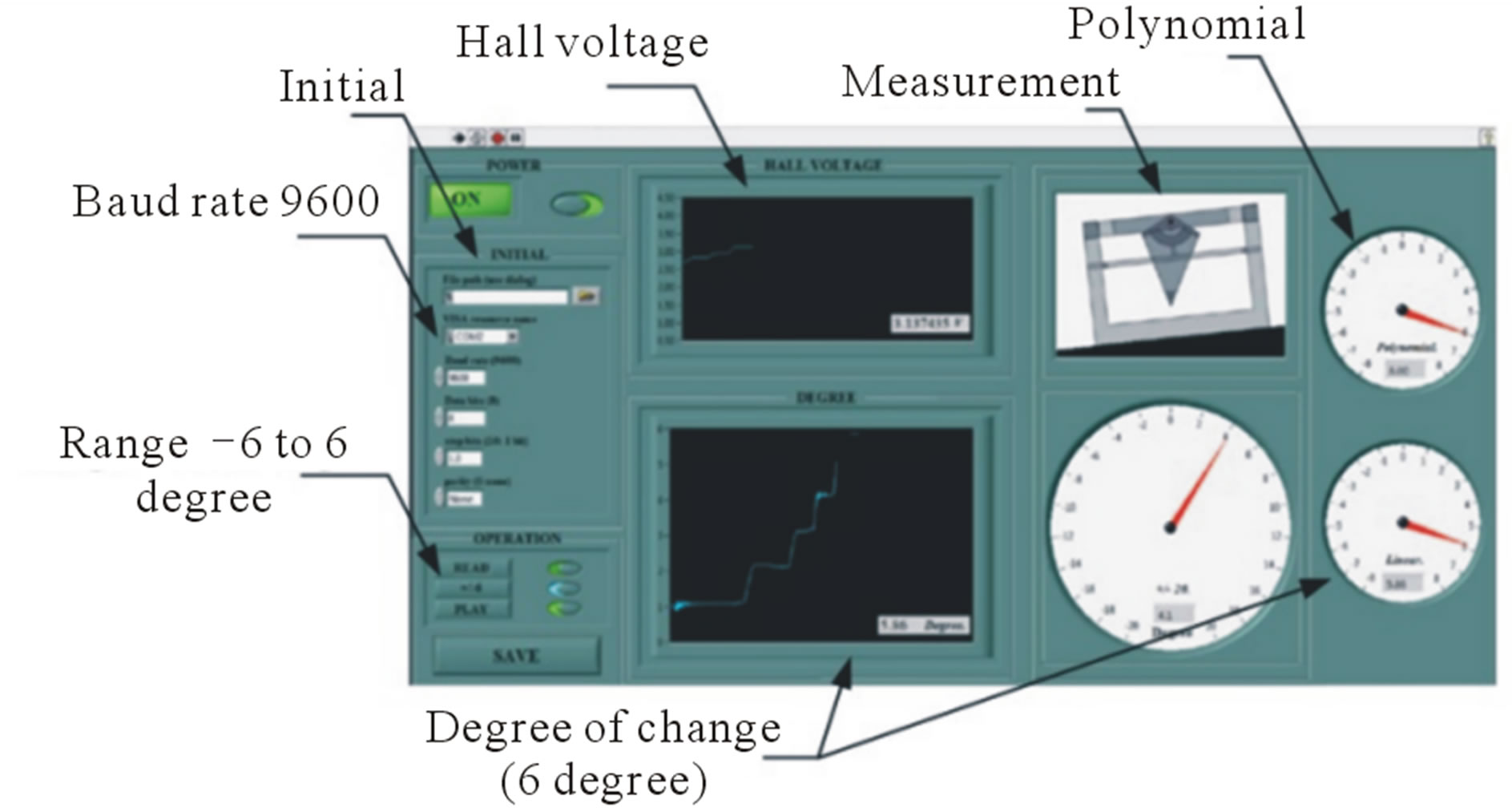
Figure 12. Experiment of 6 degree.

Figure 13. Experiment of the range of 20 degree.
R2 is regression value.
5.1. Analysis of –20 to 20 Degree
Analysis of inclined angle using LSSM which tilting away on X-axis in both (+) and (–) direction was considered in the range of 0 to ±20 degree (normal to Y-axis) with 1 degree of resolution per step as shown in Figure 15. To analyze the density of magnetic field at any position within the flat-curve permanent magnetic plate radius, the module system was angularly moved on the X-axis starting from the reference point (0 degree). The measured results were presented in output voltage which varied by the current flowing through the HES and dependent on magnetic field density. Moreover, the output voltage of HES was also dependent on the density and direction of magnetic field which varied from –20 degree (1.157 Volt) to 20 degree (3.829 Volt).
Experimental results can be used for analysis of the relationship of output voltage from HES and magnetic field density at the tilted position of sensing module on X-axis as showing in Figure 16. The results agreed well to the results from calculation using COMSOL software simulation. The space between two flat-curve permanent magnets was equal to 12 mm. However, the system developed can be expressed by the variation of output

Figure 14. Relationship of output voltage from HES and magnetic field density (–40 to 40 degree).

Figure 15. LSSM inclination on X-axis (–20 to 20 degree).
voltage through a third degree polynomial as given in Equation (7) and the regression value is provided in Equation (8)
y = –0.0001x3 + 0.0067x2 – 0.0341x + 1.2336 (7)
R² = 0.9993 (8)
Considering the angle of LSSM inclination by repeatedly measuring 15 values and then comparing to actual values, it can be noted that the measured inclination angle exhibited the results with high accuracy and reliability at any angle in the range between –20 to 20 degree. From Figure 16, it can be observed that the range with the best linearity was –10 degree to 10 degree because the position of HES was mostly close to permanent magnets and the magnetic density can reach the maximum at this position. Therefore, the range of –10 degree to 10 degree was practically used. The output voltage as a function of inclined angle change for every single degree can be provided as shown in Table 1.

Figure 16. Relationship of output voltage from the HES and magnetic field density (–20 to 20 degree).
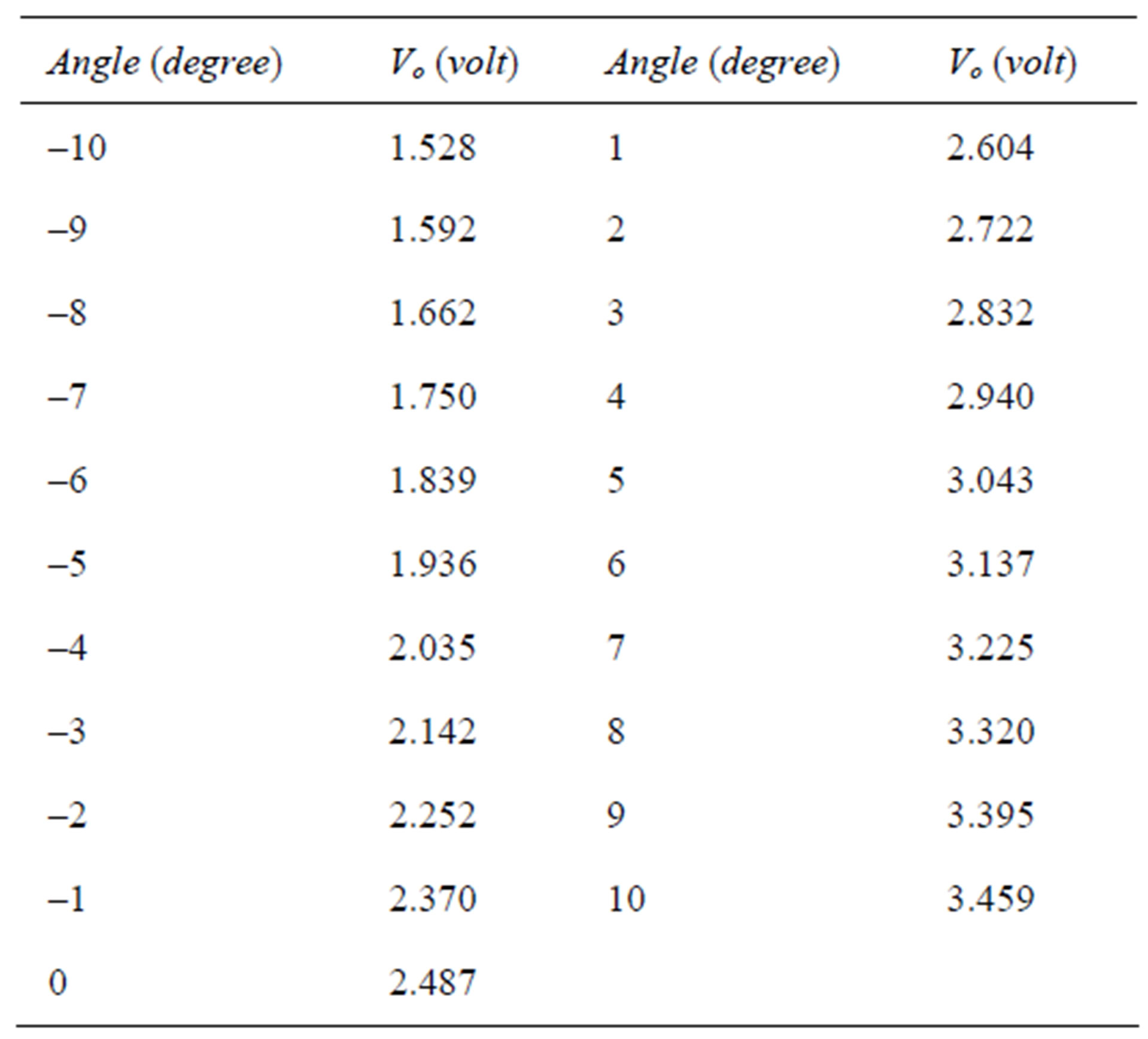
Table 1. Output voltage as a function of inclined angle in the range of –10 to 10.
From Table 1, it can be noted that the relationship of output voltage and inclined angle can provide the best linearity of the results in the range of –6 degree to 6 degree for the resolution of 100 mV per 1 degree. Use of the monitoring system developed to observe ground level subsidence or to setup industrial machines would provide high accuracy and reliable in this range.
5.2. Analysis of –6 to 6 Degree
Considering angular analysis of the range of –6 to 6 degree by using LSSM developed, it was found that the results were similar to the range of –20 to 20 degree with 0.01 degree of resolution per step as shown in Figure 17. In this case, the output voltage of HES was also dependent on the density and direction of magnetic field which varied from –6 degree (1.839 Volt) to 6 degree (3.137 Volt).
The experimental results of the relationship between output voltage from HES and magnetic field density in any inclined position of LSSM can be used analysis is as shown in Figure 18. The linear relationship of output voltage from HES on X-axis and inclined angle on Y-axis as function of magnetic field variation is as given in Equation (9) and the regression value is provided in Equation (10).
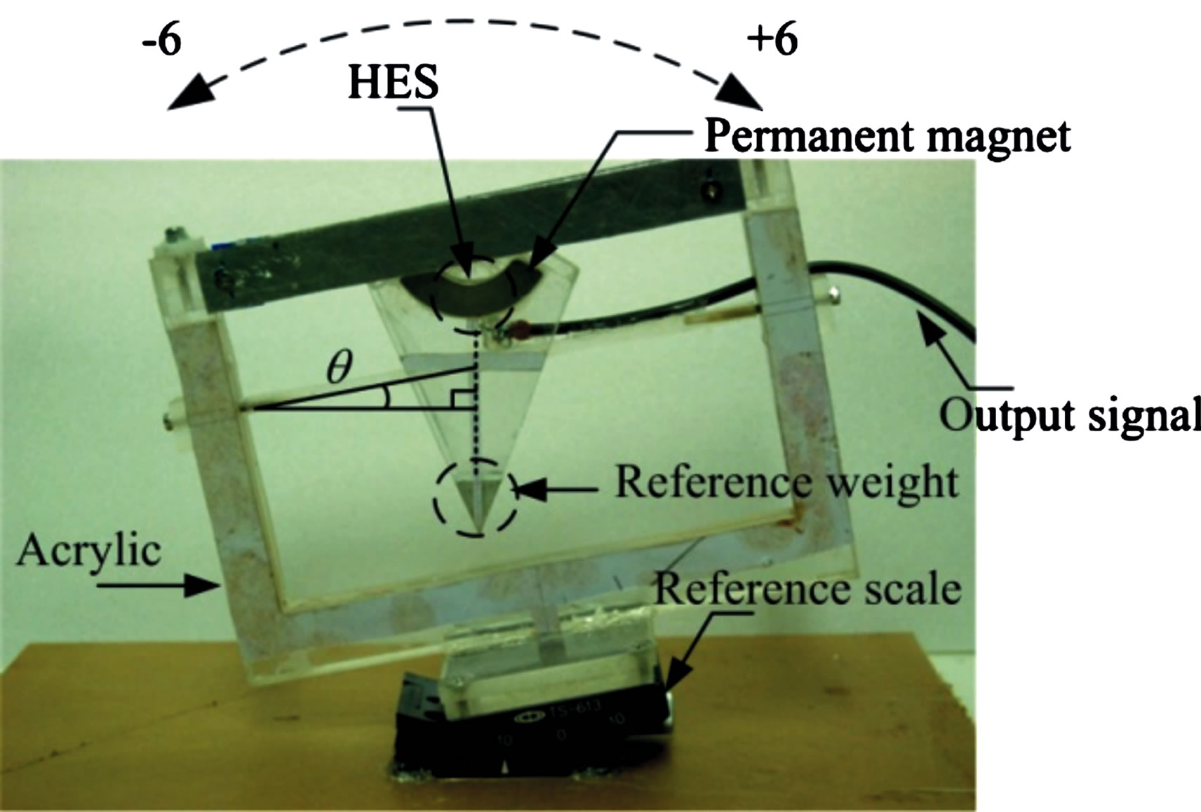
Figure 17. LSSM inclination on X-axis (–6 to 6 degree).

Figure 18. Relationship of output voltage from the HES and magnetic field density (–6 to 6 degree).
y = 0.1098x + 1.7168 (9)
R2 = 0.9991(10)
When repeatedly measuring 15 values, it was observed that the range of –6 to 6 degree exhibited the results with high resolution, high accuracy, and high reliability throughout experiment. From experimental study, accuracy, precision, and reliability were analyzed by considering the mean value and standard deviation (STD) as shown in Table 2. In analysis of the output voltage from HES, it can be observed that the inclination of LSSM at any position within the flat-curve permanent magnets radius would exhibit the best accuracy of 99%.
6. Conclusion
From analysis of magnetic field density variation on HES due to inclined angle change, it can be noted that any point of permanent magnet formally generates the different magnetic density. Therefore, the output voltage from HES can be used to determine the angle of inclination. The experiments were separated in two ranges: the range of –20 to 20 degree and the range of –6 to 6 degree. The monitoring system developed (LSSM) can provide the results with the best accuracy and reliability for observing ground level subsidence or industrial machine

Table 2. Mean and standard deviation for within the range of –6 to 6 degree.
alignment for the inclined angle within the range of –6 to 6 degree with 0.01 degree of resolution per step. Moreover, the LSSM can be applied to monitor the level of land subsidence in the area of the industrial machine located such as industrial machine alignment and installation as well as to examine the inclination of structure in civil engineering.
REFERENCES
- V. Hiligsmann and P. Riendeau, “Monolithic 360 Degrees Rotary Position Sensor IC,” IEEE Sensors Conference, Vienna, 24-27 October 2004, pp. 1137-1142.
- B. Lequesne and T. Schroeder, “High-Accuracy Magnetic Position Encoder Concept,” IEEE Transactions on Industry Applications, Vol. 35, No. 3, 1999, pp. 568-576. doi:10.1109/28.767003
- Y. Y. Lee, R. H. Wu and S. T. Xu, “Applications of Linear Hall-Effect Sensors on Angular Measurement,” 2011 IEEE International Conference on Control Applications (CCA), Denver, 28-30 September 2011, pp. 479-482. doi:10.1109/CCA.2011.6044465
- G. Arfken, “Mathematical Methods for Physicists,” Academic Press, Orlando, 1985.
- C. Chaiyachit, S. Satthamsakul, W. Sriratana and T. Suesut, “Hall Effect Sensor for Measuring Metal Particles in Lubricant,” International Multi Conference of Engineers and Computer Scientists 2012 (IMECS 2012), Hong Kong, 14-16 March 2012, pp. 894-897.
- L. Tanachaikhan, N. Tammarugwattana, W. Sriratana and P. Klongratog, “Declined Angle Analysis of Shaft Using Magnetic Field Measurement,” ICROS-SICE International Joint Conference 2009, Fukuoka International Congress Center, Fukuoka, 18-21 August 2009, pp. 1846- 1849.
- E. Ramsden, “Hall-Effect Sensor: Theory and Applications,” Elsevier, Burlington, 2006.
- United Kingdom Accreditation Service, “The Expression of Uncertainty and Confidence in Measurement,” United Kingdom Accreditation Service, London, 1997.
- W. Sriratana, R. Murayama and L. Tanachaikhan, “Application of the HES in Angular Analysis,” Journal of Sensor Technology, Vol. 2 No. 2, 2012, pp. 87-93. doi:10.4236/jst.2012.22013
- W. Sriratana, K. Nakmee and L. Tanachaikhan, “Subsidence Monitoring System for Industrial Machines Based on Magnetic Field Method,” International Conference on Control, Automation and Systems 2010 (ICCAS 2010), Seoul, 27-30 October 2010, pp. 346-349.