Natural Science
Vol.6 No.2(2014), Article ID:43146,10 pages DOI:10.4236/ns.2014.62011
The quantum thermodynamic functions of plasma in terms of the Green’s function
1Mathematics Department, Assuit University, Assuit, Egypt
2Mathematics Department, South Valley University, Qena, Egypt
3Mathematics Department, Assiut University, New Valley, Egypt; *Corresponding Author: dalia_ah@yahoo.com
Copyright © 2014 Nagat A. Hussein et al. This is an open access article distributed under the Creative Commons Attribution License, which permits unrestricted use, distribution, and reproduction in any medium, provided the original work is properly cited. In accordance of the Creative Commons Attribution License all Copyrights © 2014 are reserved for SCIRP and the owner of the intellectual property Nagat A. Hussein et al. All Copyright © 2014 are guarded by law and by SCIRP as a guardian.
Received 30 November 2013; revised 30 December 2013; accepted 7 January 2014
Keywords:The Excess Free Energy; The Two Component Plasma; The Third Virial Coefficient; The Hartree Term; The Hartree-Fock Approximation
ABSTRACT
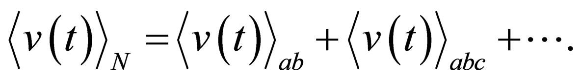
The objective of this paper is to calculate the third virial coefficient in Hartree approximation, Hartree-Fock approximation and the MontrollWard contribution of plasma by using the Green’s function technique in terms of the interaction parameter
 , and used the result to calculate the quantum thermodynamic functions for one and two component plasma in the case of
 , where
  is the thermal De Broglie wave-length. We compared our results with others.
1. INTRODUCTION
The thermodynamic functions are of great interest for understanding the properties of plasma such as the excess free energy and the pressure. An accurate description of the pressure, volume and temperature (P-V-T) behavior represents one of the most important goals of statistical thermodynamics. Besides simulations, the equilibrium behavior can be determined either from the equation of state (EOS) or from virial expansion. The properties and the behavior of many particle systems with Coulomb interactions are essentially determined by the long range character of the forces between the charged particles. Therefore, systems with Coulomb interactions are of special interest and importance in statistical physics [1].
Many authors have calculated the excess free energy, Ebeling et al. [2] have calculated the virial expansion of the excess free energy until the second virial coefficient from the pair distribution function. Hussein and Eisa [1] calculated the quantum excess free energy for two component plasma. All these researches are used the method of Slater Sum in quantum statistical mechanics. Also, the thermodynamic functions which are calculated from these researches near to the classical limit. In this paper we use the Green’s function technique, which means that we have to start from the grand canonical ensemble. To our knowledge, no attempt to find the thermodynamic function until third virial coefficient by using Green’s function technique for one and two component plasma. The method of Green’s functions is one of the most powerful techniques in quantum statistical physics and quantum chemistry. The main advantage of Green’s functions is that one can formulate exact equations of approximations and set up consequent schemes to gain any higher approximation [3]. Another advantage of such Green’s functions is the existence of highly effective methods for their determination, such as Feynman diagram techniques, functional techniques and the formulation of equations of motion [4]. The single particle Green’s function in fact contains more detailed information than the total energy alone, to the extent that the local Slater correlation potential can be obtained from it [5]. Many authors used the method of Green’s functions such as Dewitt et al. [6] and have calculated the low density expansion of the equation of state for a quantum electron gas. Riemann et al. [7] have calculated the equation of state of the weakly degenerate one-component plasma (OCP).
The model under consideration is the two-component plasma (TCP); i.e. neutral system of point like particles of positive and negative charges which antisymmetric with respect to the charges  and therefore symmetrical with respect to the densities
 . Also, we used the one component plasma model (the model of identical point charges immersed in a uniform background, while the continuous charge density of the background is chosen to be equal and opposite to the average charge density of the point charges, so that the system as a whole is electrically neutral) for example the electron gas
  and therefore symmetrical with respect to the mass
 .
.
This paper is organized as follows: In Section 2, we present the Green’s function. In Section 3, we calculate the excess free energy until the third virial coefficient for one and two component plasma in quantum form. Also, we calulate the general formula of the third virial coefficient in Hartree-Fock approximation. Finally, in Section 4, we calculate the pressure for one and two component plasma until the third virial coefficient.
2. THE GREEN’S FUNCTION
The n-particle Green’s function is defined by [8] in the following form
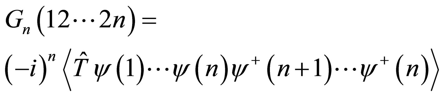 (1)
(1)
where,
 (2)
(2)
 (3)
(3)
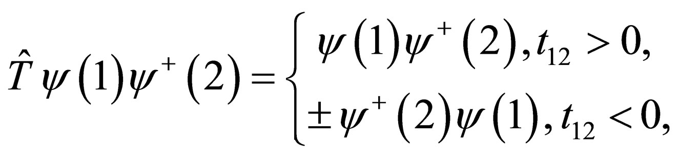
 is the time-ordering operator and
  with
with  is the vector of location,
  is time,
  is
is
 -projection of spin.
So we can defined the greater and lesser Green’s function by
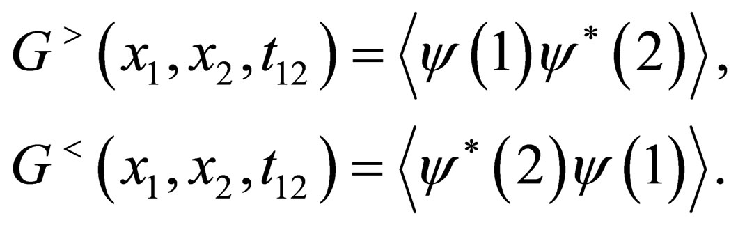 (4)
(4)
In the Hartree and the Hartree-Fock approximation the two particle Green’s function is given by
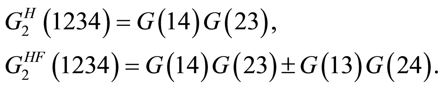 (5)
(5)
Or the variational representation [8]
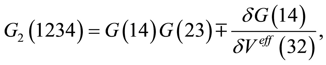 (6)
(6)
where the polarization function 
and  is the effective potential.
Also the three particle Green’s function is defined by [8]
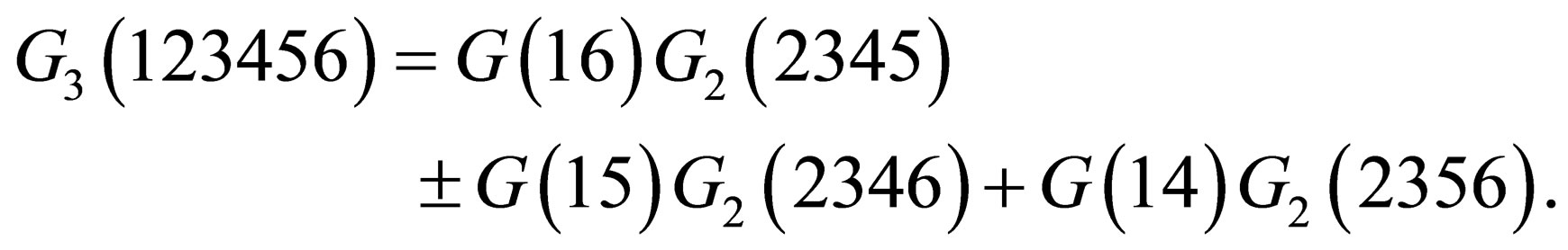 (7)
(7)
3. THE EXCESS FREE ENERGY
The excess free energy corresponds to the part of the free energy change in the real system that arises from interactions among ions [9]. The excess free energy  can be calculated from the mean value of the potential energy according to a general quantum statistical formula with the coupling parameter
  in the following form [10]
 (8)
(8)
where
 (9)
(9)
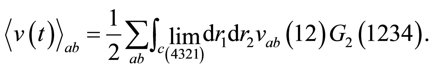 (10)
(10)
(11)
 (11.a)
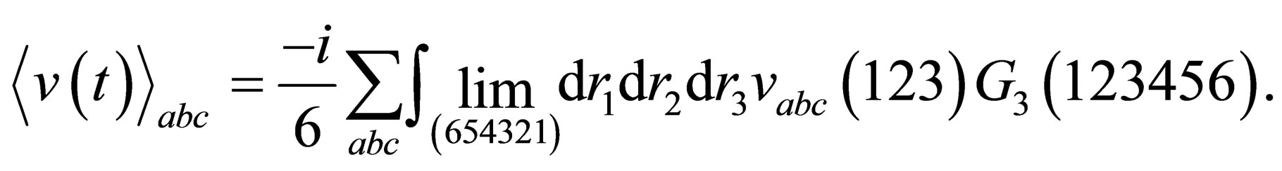
 and
and  are the mean interaction potential for two and three particle respectively.
After performing the integration with respect to  in Equation (8) we can get
 (12)
(12)
where the second virial coefficient is given by [4]

(13)
and
 (14)
(14)
Now we will calculate the third virial coefficient; for Coulomb systems it is useful to apply, instead of , the screened potential
  in Eq.14 for three particle which is given by the following form
 (15)
(15)
Then we can get the Eq.14 in the form
 (16)
(16)
where,
 (17)
(17)
(18)
and

(19)
 (20)
(20)
where are the binary potential, the triplet potential, the triplet screened potential, the triplet polarization function, one particle Green’s function, the two particle Green’s function in Hartree approximation, the three particle Green’s function, the triplet Hartree term, the triplet Hartree-Fock, the triplet screened respectively.
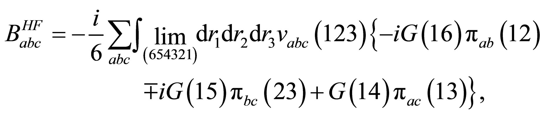
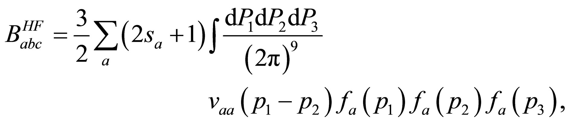
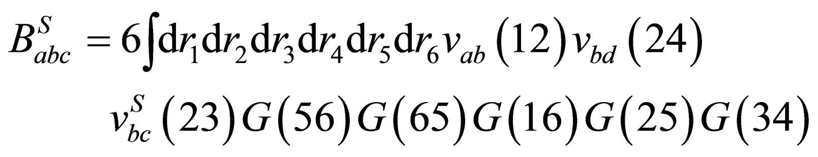
3.1. The Hartree Term of Babc
By substituting from Eq.5 and 7 into Eq.17 then the Hartree term of the quantum third virial coefficient  becomes
 (21)
(21)
By taking the inverse Fourier transformation of the above equation and making use of the Wigner distribution function [4];
 (22)
(22)
and using Equation (20) we obtain
 (23)
(23)
where the number density
 (24)
(24)
Eq.23 is vanishes for example for one component plasma such as the electron gas.
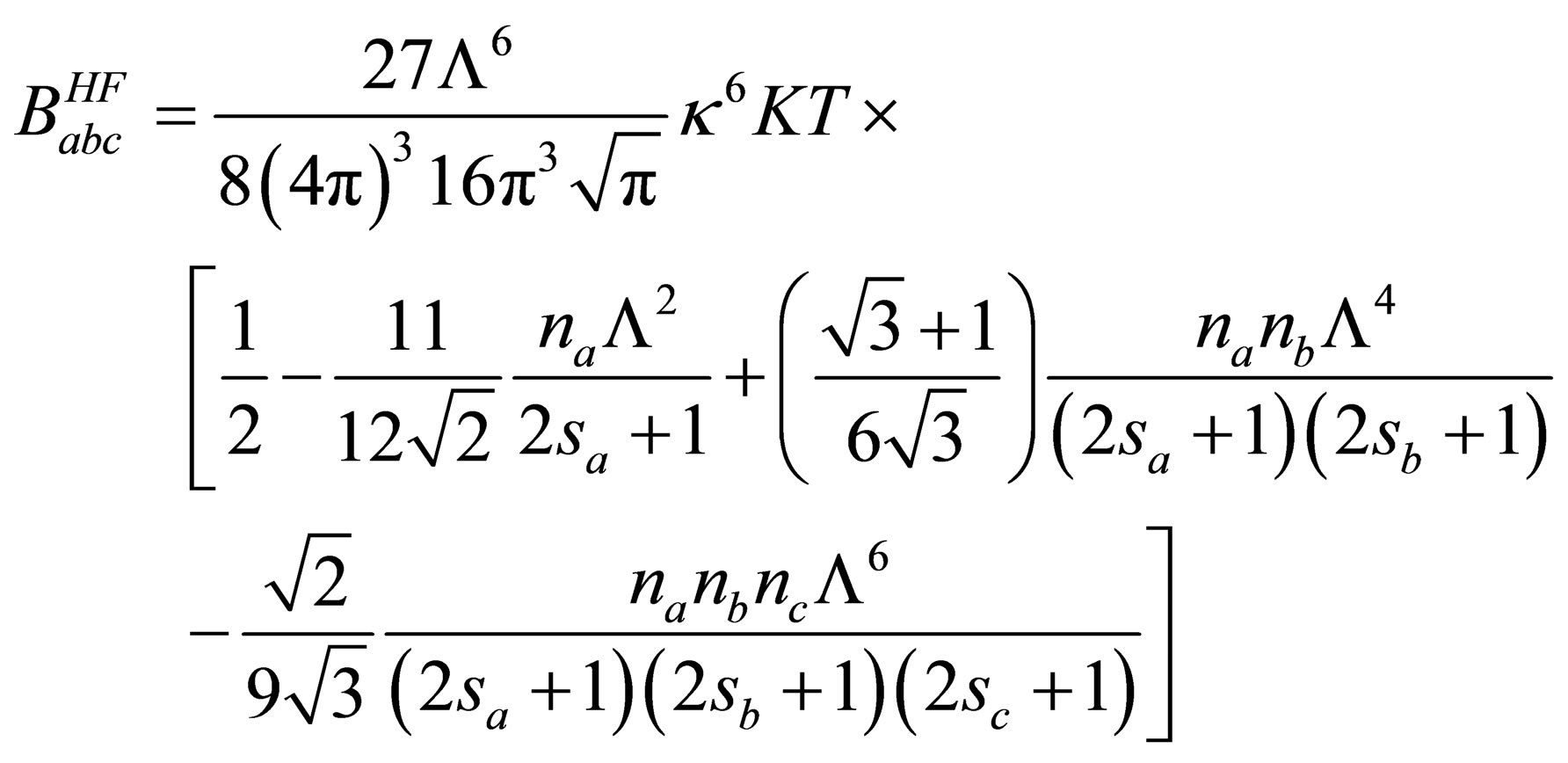
3.2. The Hartree-Fock Term of Babc
The polarization function is defined random phase approximation by
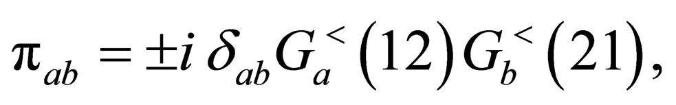 (25)
(25)
By substituting from Eq.25 into Eq.18 we can get the Hartree-Fock term of the quantum third virial  as follow
 (26)
(26)
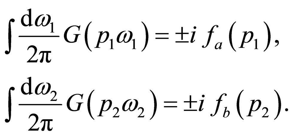
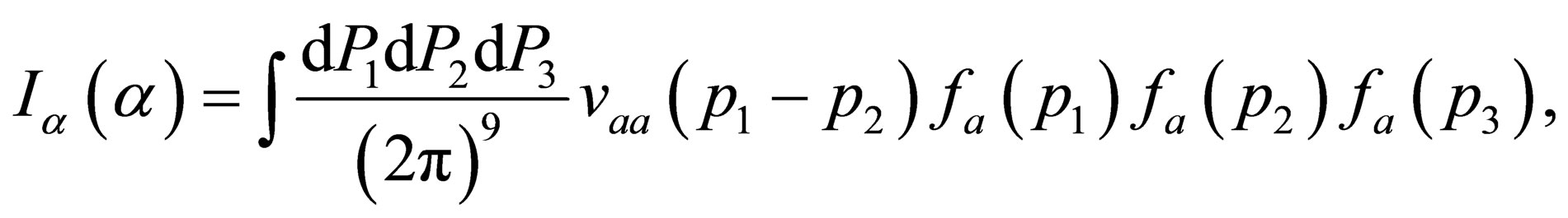
The inverse Fourier transform of this equation with the help of the Eq.22 gives
(27)
where,  and
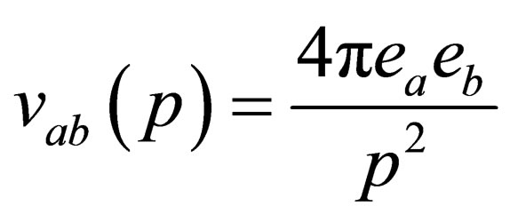
and  are Fermi functions and the Fourier transform of Coulomb potential which is defined by
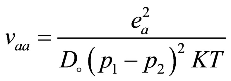 (28)
(28)
with  is the dielectric constant where
  are the vacuum and the relative dielectric constant.
We assume that
(29)
By expanding  and
and  in powers of
  and using the spherical polar coordinates (see Appdenix A) then

(30)
Then
 (31)
(31)
let
 (32)
(32)
The calculation of  analytically, gives
 (33)
(33)
By substituting from Eq.33 into Eq.31 then we get
 (34)
(34)
where, 

 and
and  are the Fermi integral, the volume, the spin projection, the degeneracy parameter, the chemical potential, the Boltzmann’s constant and the absolute temperature respectively.
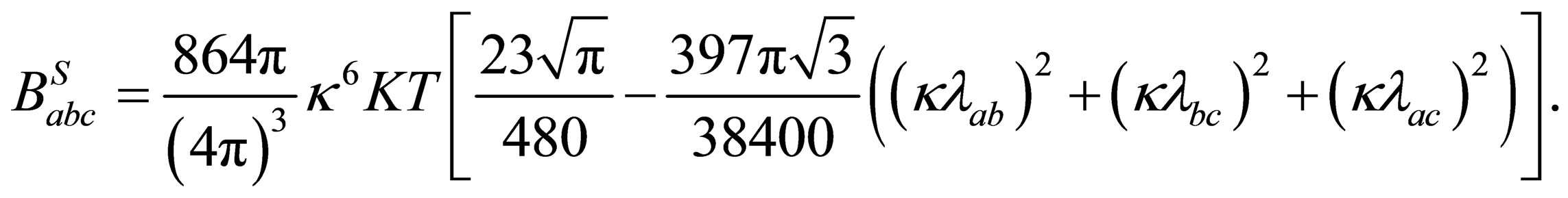
Then we can written the third virial coefficient in the following form
(35)
3.3. The Screened Contribution of Babc
By substituting from Eqs.6 and 7 into Eqs.19 we can rewrite the screened quantum third virial  until first three terms in the following form
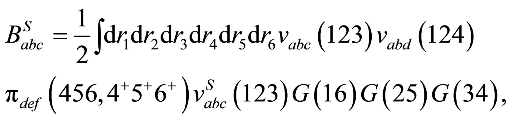 (36)
(36)
by using the pair potential and pair polarization function then
 (37)
(37)
Taking the inverse Fourier transformation of Eq.37 and using Eq.20, where
is the Fourier transform of binary potential then we get in the weakly degenerate case or low degeneracy limit  and the case of high temperature limit or low density
  in the following form
 (38)
(38)
where  is the inverse Debye length and
  denotes the confluent hypergeometric function.
The analytical calculation of the integral from Eq.38 is evaluated by solving this integral by parts and using Gamma functions in the regions of small  (low densities, high temperatures) then we have
 (39)
(39)
By substituting from Eqs.13, 23, 35 and 39 into Eq.12 we get the excess free energy until the third virial coefficient for one component plasma as follow
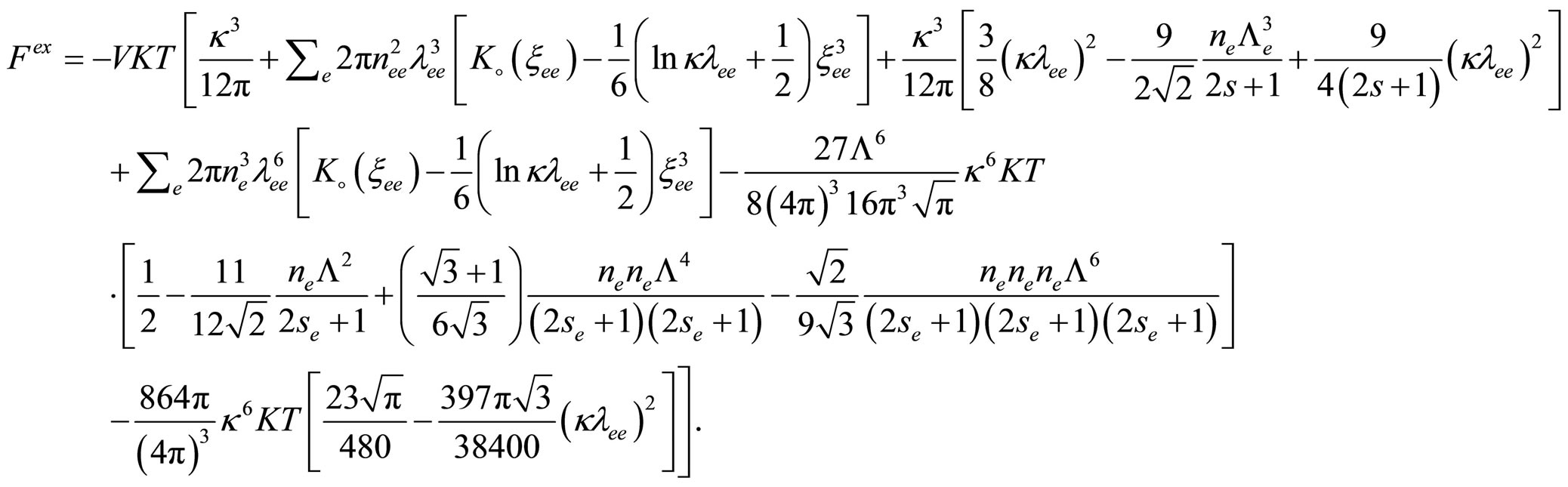 (40)
(40)
where  is the quantum virial function which given by [4] and
  is the normalized thermal wave length.
Similarly, we can write the excess free energy until the third virial coefficient for two component plasma as follow
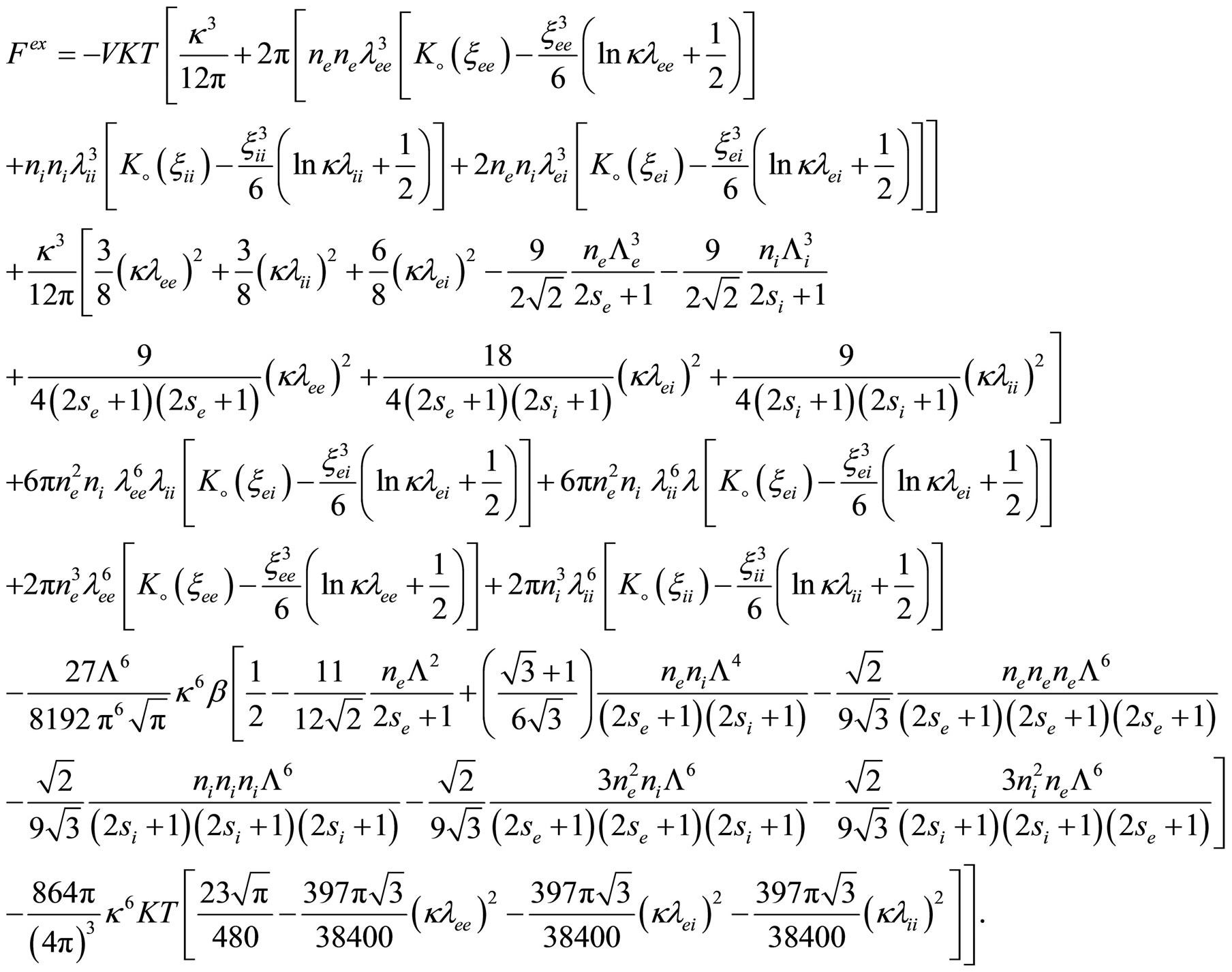 (41)
(41)
4. THE EQUATION OF STATE
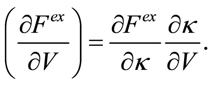
Following the method of effective potentials developed by [9] we get the pressure from the excess free energy as follow
 (42)
(42)
where  is the ideal pressure and
By substituting from Eq.40 into Eq.42 we can get the equation of state until third virial coefficient for one component plasma;
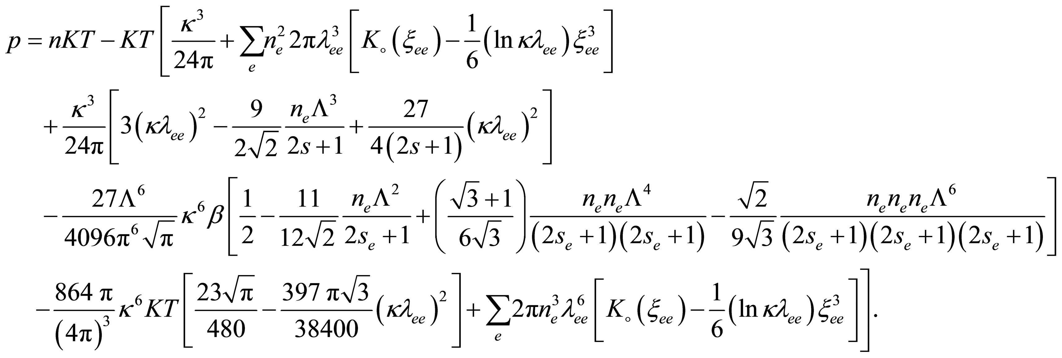 (43)
(43)
Also, by substituting from Eq.41 into Eq.42 we get the equation of state until third virial coefficient for two component plasma
 (44)
(44)
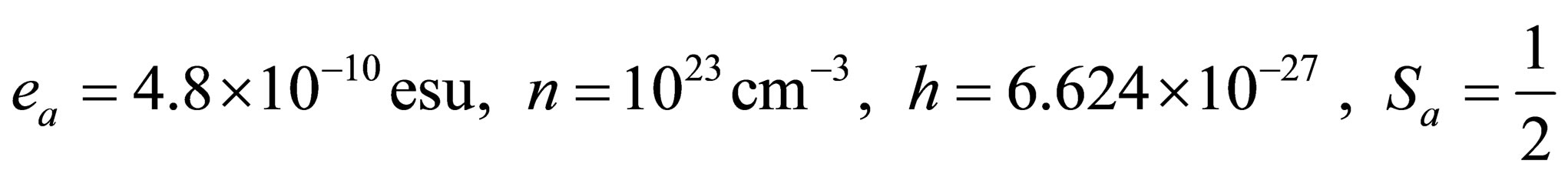
In the numerical calculation, we let

5. DISCUSSIONS
To our knowledge there is no paper to calculate the third virial coefficient by using Green’s function technique until now; this paper is the first paper to calculate the third virial coefficient in Hartree, Hartree-Fock approximation and the Montroll-Ward contribution by using the Green’s function technique, and used it to calculate the quantum thermodynamic functions. In past the potential was used as the mean potential for two particles only so their results were until the second virial coefficient, but in this paper we used the potential as the sum of the mean potential of two and three particles so our results were evaluated until the third virial coefficient. Also the quantum thermodynamic functions until the third virial coefficient which are calculated by using the binary Slater sum are near at the classical limit only; they used the potential as the pair potential only and neglected the triplet potential so there results Is not exactly correct results. We considered only the thermal equilibrium plasma in the case of one and two component plasma by using Green’s function method. We obtained the general formula of the third virial coefficient in Hartree-Fock approximation analytically (Eq.34).
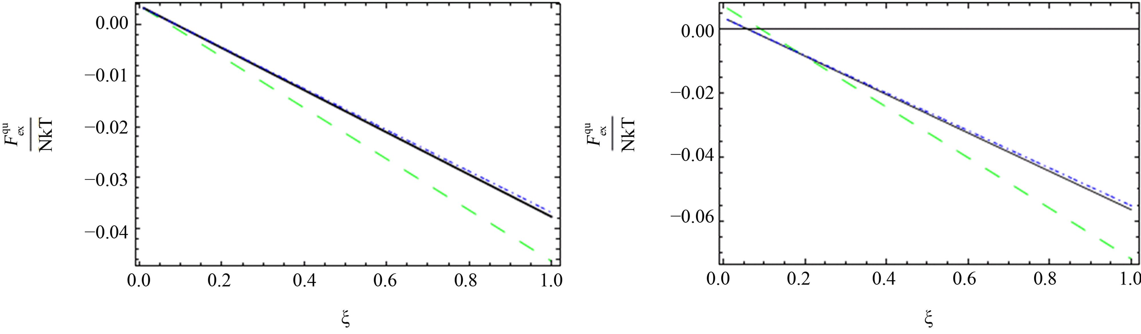
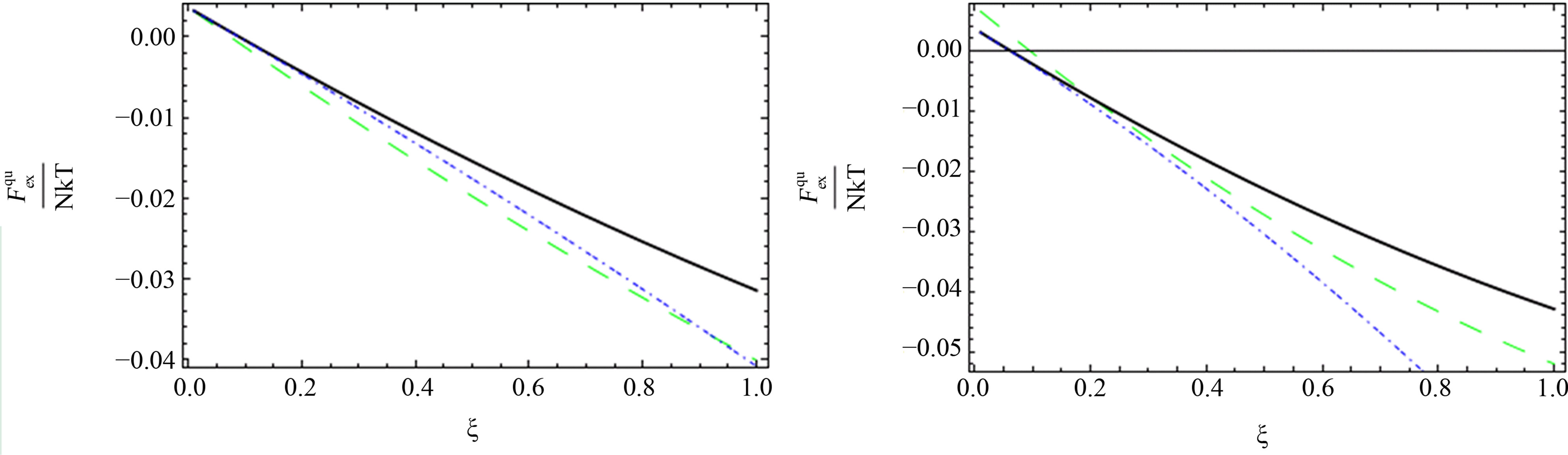
As shown in Figures 1-3, we plotted the comparison between the excess free energy until the second virial coefficient for one and two component plasma of Ebeling et al. [11], Hussein et al. [1] until the third virial coefficient and our results until the third virial coefficient at  and
and . We noticed that the curves are small nearly for small values of
 , this is due to the difference between Green’s function technique which was used here and Slater Sum technique in Hussein et al. [2] and Ebeling et al. [11] which are given in Figures 1-3. In these figures we observe that there exist difference for small values of
  for two comopnent plasma especially order
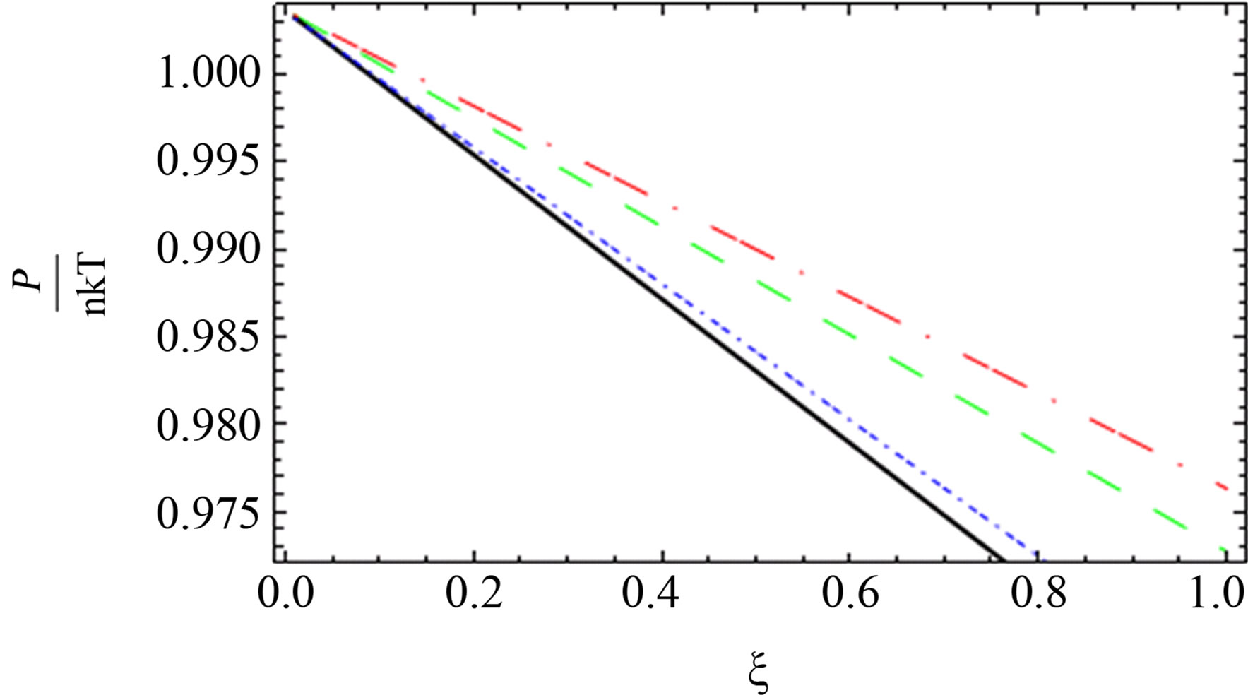
 . Also, we plotted the comparison between the pressure until the second virial coefficient for one and two component plasma of Kremp et al. [4], Ebeling et al. [11], Hussein et al. [1] until the third virial coefficient and our results until the third virial coefficient up to order
  and
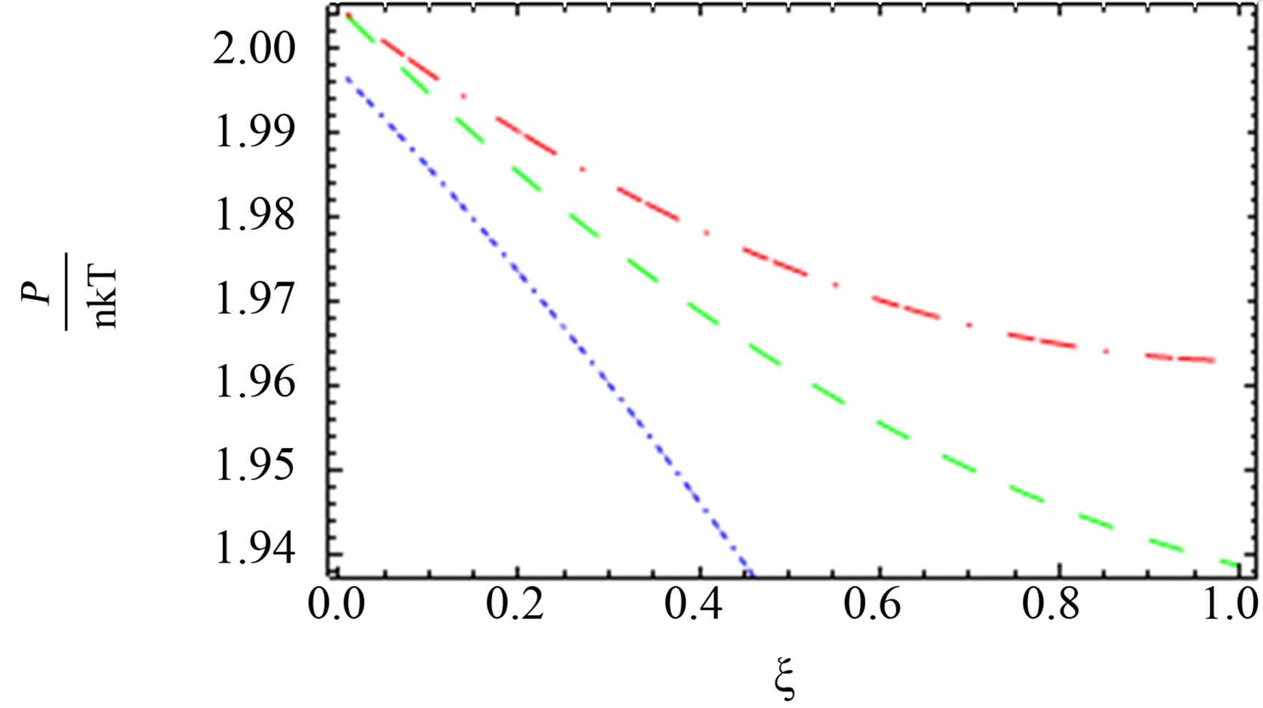
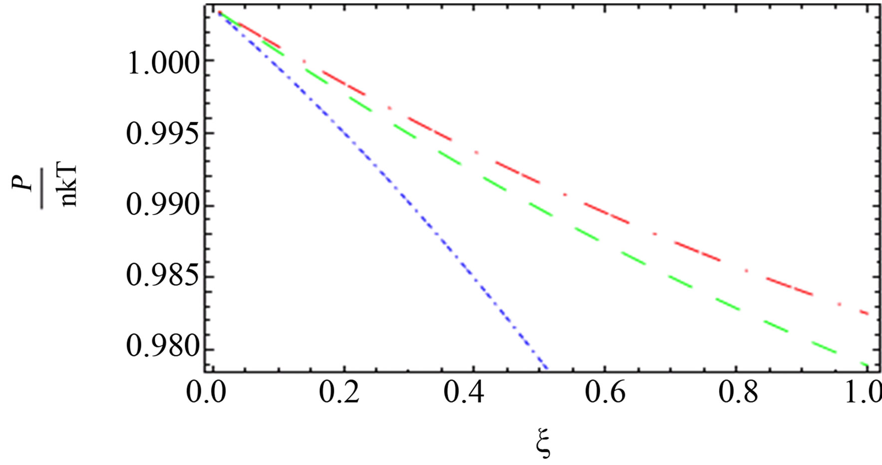
and  as shown in Figures 4-6. In Figures 5 and 6, the curves are far from each other for one and two component plasma. But in Figure 4, we observed that the red curve for Ebeling et
(a) one component plasma (b) two component plasma
Figure 1. The comparison between the quantum excess free energy until the second virial coefficient [11] (black solid line), [1] (blue short dashed dotted line) until the third virial coefficient and our results (green long dashed line) up to order e2.
(a) one component plasma (b) two component plasma
Figure 2. The comparison between the quantum excess free energy until the second virial coefficient [11] (black solid line), [1] (blue short dashed dotted line) until the third virial coefficient and our results (green long dashed line) up to order e4.

(a) one component plasma (b) two component plasma
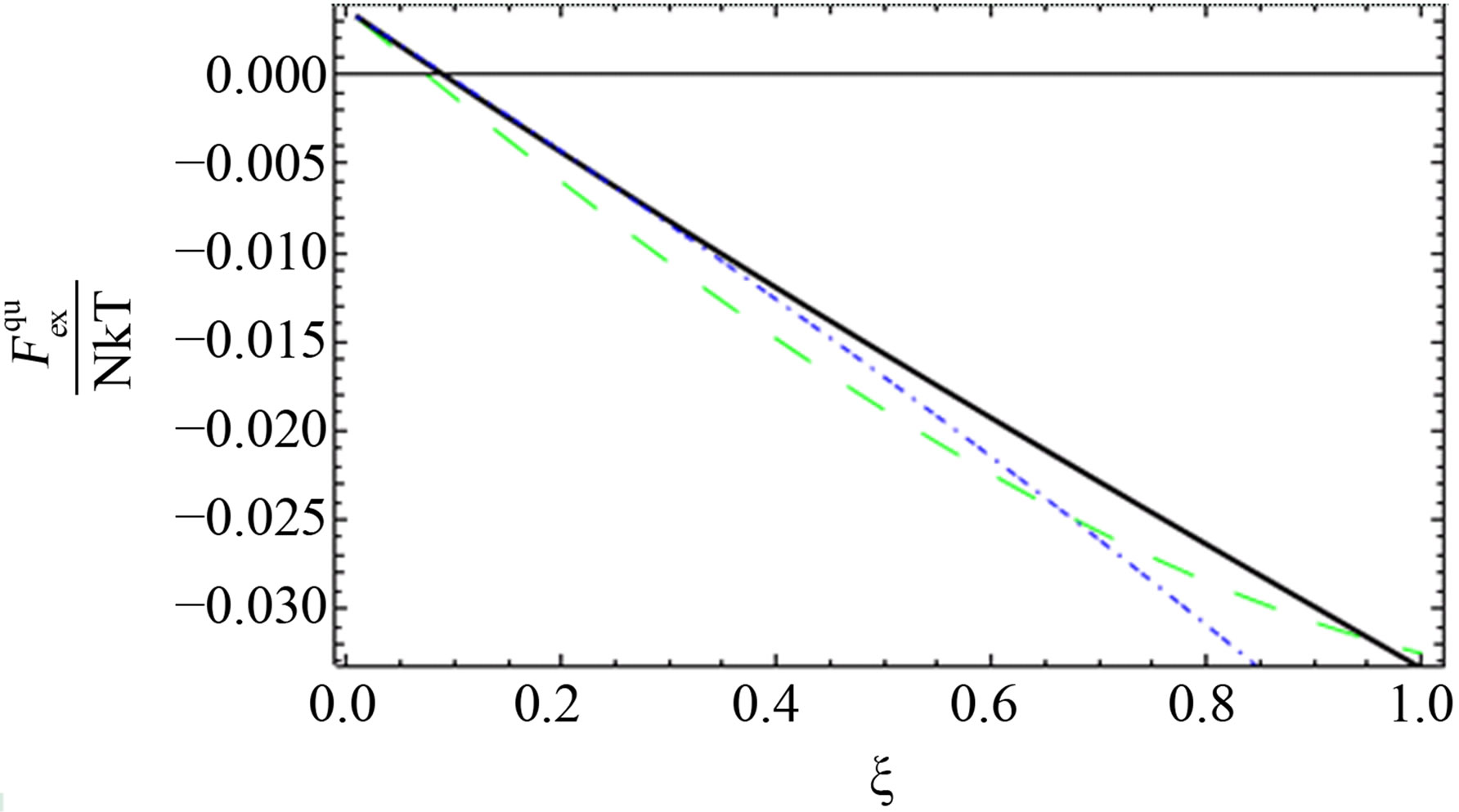
Figure 3. The comparison between the quantum excess free energy until the second virial coefficient [11] (black solid line), [1] (blue short dashed dotted line) until the third virial coefficient and our results (green long dashed line) up to order e6.
(a) one component plasma (b) two component plasma
Figure 4. The comparison between the quantum pressure until the second virial coefficient [11] (black solid line), [4] (red long dashed dotted line) and [1] (blue short dashed dotted line) until the third virial coefficient and our results (green long dashed line) up to order e2.

(a) one component plasma (b) two component plasma
Figure 5. The comparison between the quantum pressure until the second virial coefficient [10] (red long dashed dotted line), [1] (blue short dashed dotted line) until the third virial coefficient and our results (green long dashed line) up of order e4.
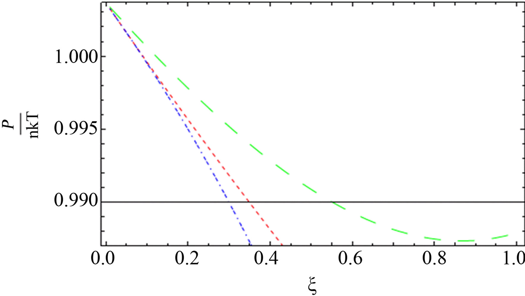
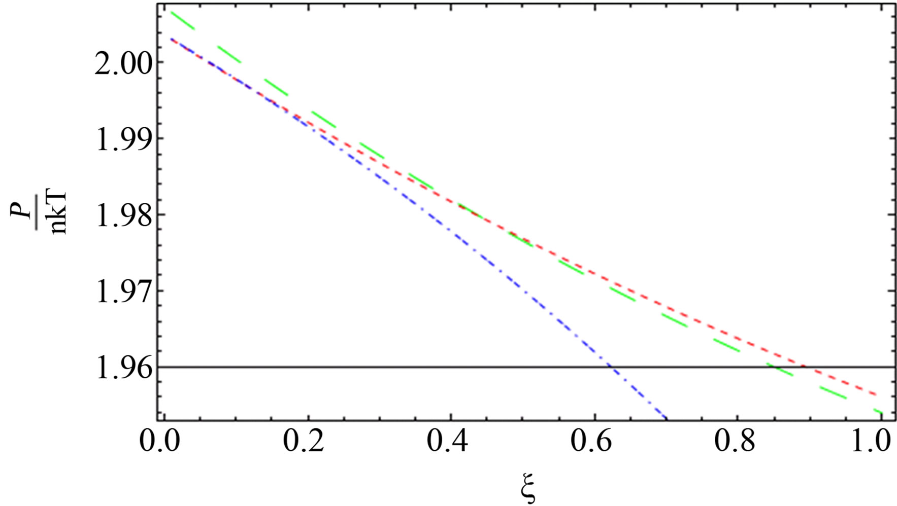
Figure 6. The comparison between the quantum pressure until the second virial coefficient (red dotted line), [1] (blue short dashed dotted line) until the third virial and our result (green long dashed line) up to order e6.
al. [11] and green curve for our result are nearly for some values of  for two component plasma.
REFERENCES
- Hussein, N.A. and Eisa, D.A. (2011) The quantum equation of state of fully ionized plasmas. Contributions to Plasma Physics, 51, 44-50. http://dx.doi.org/10.1002/ctpp.201110003
- Ebeling, W. (1966) Zur freien energie von systemen geladener teilchen. Annalen der Physik, 472, 415-416. http://dx.doi.org/10.1002/andp.19664720709
- Kraeft, W.D. and Fehr, R. (1997) Self energy and two particle states in dense plasmas. Contributions to Plasma Physics, 37, 173-184. http://dx.doi.org/10.1002/ctpp.2150370209
- Kremp, D., Schalanges, M. and Kraeft, W.D. (2005) Quantum statistics of non ideal plasma. Springer, New York. http://www.springer.com/978-3-540-65284-7
- Holleboom, L.J., Snijders, J.G., Baerends, E.J. and Buijse, M.A. (1988) A correlation potential for molecular systems from the single particle Green’s function. The Journal of Chemical Physics, 89, 3638. http://dx.doi.org/10.1063/1.454884
- Dewitt, H.E., Schlanges, M., Sakakura, A.Y. and Kraeft, W.D. (1995) Low density expansion of the equation of state for a quantum electron gas. Physics Letters A, 197, 326-329. http://www.sciencedirect.com/science/article/pii/S0375960105800118 http://dx.doi.org/10.1016/S0375-9601(05)80011-8
- Riemann, J., Schlanges, M., Dewitt, H.E. and Kraeft, W.D. (1995) Equation of state of the weakly degenerate one-component plasma. Physica A, 219, 423-435. http://EconPapers.repec.org/RePEc:eee:phsmap:v:219:y:1995:i:3:p:423-435 http://dx.doi.org/10.1016/0378-4371(95)00179-B
- Yukalov, V.I. (1998) Statistical Green’s functions. Kingston, London.
- Falkenhagen, H. and Ebeling, W. (1971) Equilibrium properties of ionized dilute electrolytes. In: Falken-Hagen, H. and Ebeling, W., Eds., Ionic Interactions from Dilute Solution to Fused Salts, Academic Press, New York and London, 1-59. http://www.sciencedirect.com/science/article/pii/B9780125530019500062
- Kraeft, W.D., Kremp, D. and Ebeling, W. (1986) Quantum statistics of charged particle systems. Akademie Verlag, Berlin. http://link.springer.com/book/10.1007%2F978-1-4613-2159-0
- Hoffmann, H.J. and Ebeling, W. (1968) Quantenstatistik des Hochtemperatur-Plasmas im thermodynamischen Gleichgewicht. II. Die freie Energie im Temperaturbereich 106 bis 108 ˚K. Beitrage aus der Plasmaphysik, 8, 43-56. http://dx.doi.org/10.1002/ctpp.19680080105
APPENDIX A
By expanding  and
and  in powers of
  then
then
 (A.1)
(A.1)
where,
 (A.2)
(A.2)
by substituting by , we get
 (A.3)
(A.3)
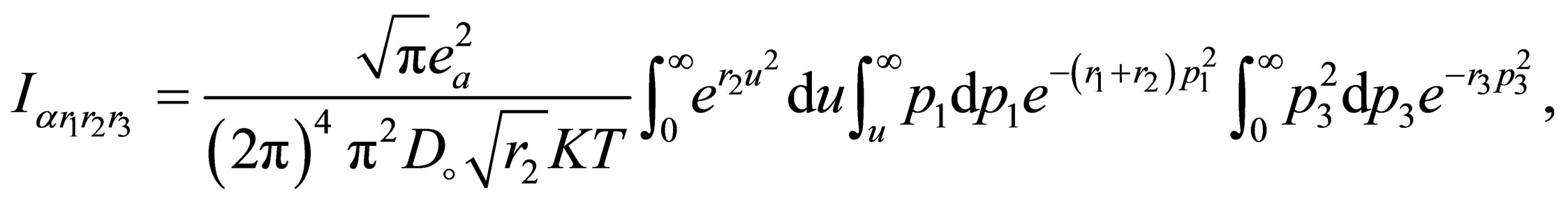
by using the integration by parts we get without Dirichlet formula
 (A.4)
(A.4)
we have the integral region  for the inner bounds, if we look at the curves
  which we want to solve in terms of
  we find that
  and finally we have
 (A.5)
(A.5)
which can be written as
 (A.6)
(A.6)