ABSTRACT

The goal of this paper is to study an output stabilization problem: the gradient stabilization for linear distributed systems. Firstly, we give definitions and properties of the gradient stability. Then we characterize controls which stabilize the gradient of the state. We also give the stabilizing control which minimizes a performance given cost. The obtained results are illustrated by simulations in the case of one-dimensional distributed systems.

1. Introduction

One of the most important notions in systems theory is the concept of stability. An equilibrium state is said to be stable if the system remains close to this state for small disturbances; and for an unstable system the question is how to stabilize it by a feedback control.

For finite dimensional systems, the problem of stabilization was considered in many works and various results have been developed [1]. In the infinite dimensional case, the problem has been treated in Balakrishnan [2], Curtain and Zwart [3], Pritchard and Zabczyk [4], Kato [5], Triggiani [6]. Many approaches have been considered to characterize different kinds of stabilization for linear distributed systems: Lyapunov and Riccati equation for exponential stabilization, and dissipative type criterion for the case of strong stabilization [3-5,7]. The problem has been also treated by means of specific state space decomposition [6]. The above results concern the state, but in many real problem the stabilization is considered for the state gradient of the considered system, which means to find a feedback control such that the gradient, when

For example the problem of thermal insulation where the purpose is to keep a constant temperature of the system with regards to the outside environment assumed to be with fluctuating temperature. Thus one has to regulate the system temperature in order to vanish the exchange thermal flux. This is the case inside a car where one has to change the level of the internal air conditioning with respect to the external temperature.

As we cannot always have external measurements, we use a sensor to measure the flux, which is a transducer producing a signal that is proportional to the local heat flux.

The purpose of this paper is the study of gradient stabilization. It is organized as follows: In the second section we define and characterize gradient stability. In the third section, we characterize gradient stabilizability, by finding a control that stabilizes the gradient of a linear distributed system and we give characterizations of such a control. In the fourth section we search the minimal cost control that stabilizes the system gradient. In the last section we give an algorithmic approach for control implementation and simulation examples.

2. Gradient Stability

This section is devoted to some preliminaries concerning definition and characterization of gradient stability for linear distributed systems.

2.1. Notations and Definitions

Let be an open regular subset of and let us consider the state-space system

(1)

where is a linear operator generating a strongly continuous semigroup, , on the state space H which is continuously embedded in.

H is endowed with its a complex inner product. and the corresponding norm.

We define the operator by:

(2)

is endowed with its usual complex inner product and the corresponding norm where:

(3)

With and where The mild solution of (1) is given by.

Let denote the adjoint operator of, and we define the operator which a bounded operator applying H into itself.

Definition 2.1

The system (1) is said to be

• Gradient weakly stable (g.w.s) if, the corresponding solution of (1) satisfies

• Gradient strongly stable (g.s.s) if for any initial condition the corresponding solution of (1) satisfies:

• Gradient exponentially stable (g.e.s) if there exist M, such that:

Remark 2.2

From the above definitions we have:

1) g.e.s g.s.s g.w.s.

2) If the system (1) is stable then it also gradient stable.

3) We can find systems gradient stable but not stable. This is illustrated in the following example.

Exemple 2.3

Let, on we consider the following system

(4)

Where and is the Laplace operator.

The eigenpairs of A are given by:

A generates a strongly continuous semigroup given by

then (4) isn’t stable but

Therefore the system (4) is g.e.s.

2.2. Characterizations

The following result links gradient stability of the system (1) to the spectrum properties of the operator A.

Let us consider the sets

and

where and are the points spectrum and the kernel of the operator A.

Proposition 2.4

1) If the system (1) is g.w.s then

2) Assume that the state space H has an orthonormal basis of eigenfunctions of A, if and, for some, for all then the system (1) is g.e.s.

Proof

1) Assume that there exists such that and there exists such that.

For, the solution of (1) is, so

hence the system (1) is not g.w.s.

2) For we have

where is the multiplicity of the eigenvalue gives:

for some

So we have the g.e.s of the system (1).

As example we consider (4). We have: and, , then the system (4) is g.e.s.

For the gradient exponential stability, we need the following lemma.

Lemma 2.5

Assume that there exists a function such that:

(5)

Then the operators are uniformly bounded.

Proof

Let us show that. Otherwise there exists a sequence, and such that is increasing without bound.

Now we have:

and the right-hand side goes to zero when.

By Fatou’s lemma when, almost everywhere.

Hence for some we can find a subsequence such that

But with (5) we have

when which is a contradiction.

The conclusion follows from the uniform boundedness principle.

Proposition 2.6

Assume that (5) is satisfied and

(6)

Then the system (1) is g.e.s if and only if

Proof

where, then, for some hence

Now we show that.

Let t₁ > 0, and there exists

such that for each then

With (4) we have

Therefore

then.

Hence for all there exists M' such that

So the system (1) is g.e.s.

The converse is immediate.

Example 2.7

The system (2) satisfies the conditions (5) and (6). Indeed:

Let, and.

We have, which implies

we can show that

We have.

Therefore the system (4) is g.e.s.

Corollaire 2.8

Under conditions (5) and (6) and assume, in addition, that there exists a self-adjoint positive operator such that:

(7)

where is a self-adjoint operator satisfying

(8)

then (1) is g.e.s.

Proof

We define the function,

For we have and

Thus By (8), we obtain.

Since is dense in H we can extended this inequality to all and the proposition 3.3 gives the conclusion.

For the gradient strong stability we have the following result.

Proposition 2.9

Assume that the equation

has a self-adjoint positive solution where is a self-adjoint operator satisfying (8). Moreover if the following condition holds

(9)

then (1) is g.s.s.

Proof

Let us consider the function:

For, we have and

we obtain By (8), and from (9), we have

Then

We deduce

(10)

From the density of in H, and the continuity of, (10) is satisfied for all. This means that the gradient of (1) is strongly stable.

3. Gradient Stabilizability

Let us consider the system

(11)

with the same assumptions on A, and B is a bounded linear operator mapping U, the space of controls (assumed to be Hilbert space), into H.

Definition 3.1

The system (11) is said to be gradient weakly (respectively strongly, exponentially) stabilizable if there exists a bounded operator such that the system

(12)

is g.w.s (respectively g.s.s, g.e.s).

Remark 3.2

1) If a system is stabilizable, then it is also gradient stabilizable.

2) Gradient stabilizability is cheaper than state stabilizability. Indeed if we consider the cost functional

and the spaces

and

Then we have and therefore

3) The gradient stabilization may be seen as a special case of output stabilization with output operator.

In the following we give the feedback control which stabilizes the gradient of the system (11), by two approaches.

The first is an extension of state space decomposition [6] and the second one is based on algebraic Riccati equation.

3.1. Decomposition Method

Let be a fixed real and consider the subsets and of the spectrum of A defined by

and

Assume that is bounded and is separated from the set in such a way that a rectifiable simple closed curve can be drawn so as to enclose an open set containing in its interior and in its exterior. This is the case, for example, where A is selfadjoint with compact resolvent, there are at most finitely many nonnegative eigenvalues of A and each with finite dimensional eigenspace.

Then the state space H can be decomposed [5] according to:

(13)

with, , and is the projection operator given by

where C is a closed curve surrounding.

The system (11) may be decomposed into the two subsystems

(14)

and

(15)

where and are the restrictions of A to and, and are such that, , and is a bounded operator on H_u.

The solutions of (14) and (15) are given by

(16)

And

(17)

where and denote the restriction of to and, which are strongly continuous semigroups generated by and.

For the system state, it is known (see [6]) that if the operator satisfies the spectrum growth assumption

(18)

then stabilizing (11) comes back to stabilize (14).

The following proposition gives an extension of this result to the gradient case.

Proposition 3.3

Let the state space satisfy the decomposition (13) and satisfy the following inequality

(19)

1) If the system (14) is gradient exponentially (respectively strongly) stabilizable by a feedback control, with, then the system (11) is gradient exponentially (respectively strongly) stabilizable using the control.

2) If the system (14) is gradient exponentially (resp strongly) stabilizable by the feedback control: with then the system (11) is gradient exponentially (respectively strongly) stabilizable using the feedback operator.

Proof

We give the proof for the exponential case. In view of the above decomposition, we have:.

Hence if satisfies (19) then for some and, we have:,.

It follows that the system (15) is gradient exponentially stabilizable taking v(t) = 0.

Let be such that, with

and there exists, M₂ > 0 such that

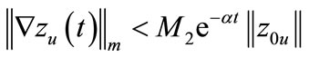
Then with the feedback control we have, with

From (17) and (18) we have

with.

Thus the system (11) excited by satisfies

which shows that the system (11) is gradient exponentially stabilizable.

2) The case of strong stabilizability follows from similar above techniques.

Corollary 3.4

Let A satisfy the spectrum decomposition assumption (13) and suppose that (19) is satisfied. If in addition 1) is a finite dimensional space 2) The system (14) is controllable on then the system (11) is gradient exponentially stabilizable.

Proof

The system (14) is of finite dimension and is controllable on the space then it is stabilizable on the same space, hence it is gradient stabilizable, the conclusion is obtained with the proposition 3.3.

3.2. Riccati Method

Let us consider the system (11) with the same assumptions on A and B. We denote by, the strongly continuous semigroup generated by, where K is the feedback operator.

Let be a self-adjoint operator such that (8) is satisfied and suppose that the steady state Riccati equation

(20)

has a self-adjoint positive solution, and let.

Proposition 3.5

1) If satisfies the conditions (5) and (6), then the system (11) is gradient exponentially stabilizable by the control

2) If then the system (11) is gradient strongly stabilizable.

3) Suppose that the system (11) is gradient exponentially stabilizable. If in addition the feedback operator K satisfiesfor some c > 0 then the state of the system (12) remains bounded.

Proof

The first and second points are deduced from the second section.

For the thirst point: Let we have

(21)

and from (21) we obtain

Since the system (11) is gradient exponentially stabilizable then, so there exists

such that for all and by the density of in H we have the conclusion.

3.3. Gradient Stabilization Control Problem

Here we explore the control that stabilizes the gradient of the system (11) as a solution of the minimization problem

(22)

where with

and R is a linear bounded operator mapping H into itself and satisfying (8).

We recall the classical result known for state stabilization if for each initial state then there exists a unique control that minimizes (22) and given by where P is a positive solution of the steady state Riccati Equation (20).

If in addition the operator R is coercive then the state of system (11) is exponentially stabilizable (see [7]).

In the following we give an extension of the above result to the gradient case.

We suppose that for each initial state, and R satisfies (8).

Proposition 3.6

The control given by minimizes where P assumed to be a self-adjoint, positive operator, and satisfies the steady state Riccati equation (20), if in addition the semigroup satisfies the conditions (5) and (6) then the same control stabilizes the gradient of system (11)

Proof

The proof follows from [7], and the proposition 3.5.

4. Numerical Algorithm and Simulations

In this section we present an algorithm which allows the calculation of the solution of problem (22) stabilizing the gradient of the system (11). By the previous result this control may be obtained by solving the algebraic Riccati Equation (20). Let where is a hilbertian basis of H. is a subspace of H endowed with the restriction of the inner product of H. The projection operator is defined by

The projection of (20) on space, is given formally by:

(23)

where, and are respectively the projections of A, P and R on, and the projection of B which is mapping U the space of control into.

We have, that is converges to P strongly in H, (see [8]).

We can write the projection of (11) like

(24)

the solution of this system is given explicitly by:

(25)

To calculate the matrix exponential we use the Padé approximation with scaling and squaring (see [9]).

If we denote, we have

(26)

Let consider a time sequence, where small enough.

With these notations, the gradient stabilization control may be obtained the algorithm steps (Table 1).

Remark 4.1

The dimension of the projection space n is choosing to be good approximation of the considered system and appropriate for numerical constraint.

Example 4.2

Let, on

which is an Hilbert space we consider the following system

(27)

where, , is the restriction operator on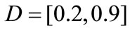, and we consider the problem (22) with.

A generates a strongly continuous semigroup

given by:, where

and with

.

The state and the gradient of system (27) are unstable since.

Let consider the subspace

Applying the algorithm taking the truncation at n = 5, we obtain figures 1 which illustrates the evolution of the system gradient and shows how the gradient evolves close to zero when the time t increases.

The gradient is stabilized with error equals 9.9836 × 10^–7 and cost equals 2.6982 × 10^–4. This shows the efficiency of the developed algorithm.

In table 2 we give the cost of gradient stabilization of system (27) for different supports control “D”.

The Table 2 shows that there is relation between area of control support and the cost of gradient stabilization, more precisely more this area decreases more cost in-

creases.

Example 4.3

Let on we consider the system (27) with Dirichlet boundary conditions:

(28)

where, , , and we consider the problem (22) with.

The eigenpairs of A are given by, , with.

The state and the gradient of system (28) are unstable since.

We consider the subspace

with.

Applying the algorithm with truncation (n = 5), the figure 2 shows the gradient evolution at times t = 3, 5, and 13.

In table 3 we present the cost of gradient stabilization

of system (28) for different zone control support “D”.

Also in this example, we remark that more the area of control support increases more the cost of gradient stabilization decreases.

4. Conclusions

In this paper the question of gradient stabilization is explored. According to the conditions, satisfied by the dynamic of system, and those satisfied by the state space, two methods are applied to characterize the controls of gradient stabilization namely, decomposition approach and Riccati method.

The obtained results are successfully illustrated by numerical simulations. Questions are still open, this is the case of regional gradient stabilization. It is under consideration and will be appear in separate paper.

5. Acknowledgements

The work presented here was carried out within the support of the Academy Hassan II of Sciences and Technology.

REFERENCES

- W. M. Wonham, “Linear multivariable Control: A Geometric Approach,” Springer-Verlag, Berlin, 1974.
- A. V. Balakrishnan, “Strong stabilizabity and the Steady State Riccati Equation,” Applied Mathematics and Optimization, Vol. 7, No. 1, 1981, pp. 335-345. doi:10.1007/BF01442125
- R. F. Curtain and H. J. Zwart, “An Introduction to Infinite Dimensional Linear Systems Theory,” SpringerVerlag, Berlin, 1995.
- A. J. Pritchard and J. Zabczyk, “Stability and Stabilizability of Infinite Dimensional Systems,” Siam Review, Vol. 23, No.1, 1981, pp. 25-51. doi:10.1137/1023003
- T. Kato, “Perturbation theory for Linear Operators,” Springer-Verlag, Berlin, 1980.
- R. Triggiani, “On the Stabilizability Problem in Banach Space,” Journal of Mathematical Analysis and Applications, Vol. 52, No. 3, 1979, pp. 383-403. doi:10.1016/0022-247X(75)90067-0
- R. F. Curtain, and A. J. Pritchard, “Infinite Dimensional Linear Systems Theory,” Springer-Verlag, Berlin, 1978.
- H. T. Banks and K. Kunisch, “The Linear Regulator Problem for Parabolic Systems,” SIAM Journal on Control and Optimization, No. 22, Vol. 5, 1984, pp. 684-696. doi:10.1137/0322043
- N. J, Higham, “The Scaling and Squaring Method for the Matrix Exponential,” SIAM Journal on Matrix Analysis and Applications, Vol. 26, No. 4, 2005, pp. 1179-1193. doi:10.1137/04061101X
- A. J. Laub, “A Schur Method for Solving Algebraic Riccati equations,” IEEE Transactions on Automatic Control, Vol. 24, No. 6, 1979, pp. 913-921. doi:10.1109/TAC.1979.1102178
- W. F Arnold and A. J. Laub, “Generalized Eigenproblem Algorithms and Soft-ware for Algebraic Riccati Equations,” Proceedings of the IEEE, vol. 72, No. 12, 1984, pp. 1746-1754. doi:10.1109/PROC.1984.13083