ABSTRACT

In quantum mechanics, there is a profound distinction between orbital angular momentum and spin angular momentum in which the former can be associated with the motion of a physical object in space but the latter cannot. The difference leads to a radical deviation in the formulation of their corresponding dynamics in which an orbital angular momentum can be described by using a coordinate system but a spin angular momentum cannot. In this work, we show that it is possible to treat spin angular momentum in the same manner as orbital angular momentum by formulating spin dynamics using Schrödinger equation in an intrinsic coordinate system. As an illustration, we apply the formulation to the dynamics of a hydrogen atom and show that the intrinsic spin angular momentum of the electron can take half-integral values and, in particular, the intrinsic mass of the electron can take negative values. We also consider a further extension by generalising the formulation so that it can be used to describe other intrinsic dynamics that may associate with a quantum particle, for example, when a hydrogen atom radiates a photon, the photon associated with the electron may also possess an intrinsic dynamics that can be described by an intrinsic wave equation that has a similar form to that for the electron.

Keywords:

Spin Angular Momentum, Spin Dynamics, Orbital Angular Momentum, Schrödinger Equation, Half-Integer Values, Intrinsic Coordinate Systems, Negative Mass

1. Introduction

In quantum physics, together with the wave-particle duality, spin angular momentum of an elementary particle is a novel dynamical feature that makes quantum mechanics stand out and be distinguished from those that are established in classical mechanics, such as the familiar orbital angular momentum. We will show in Section 2 that the profound distinction between orbital angular momentum and spin angular momentum is that the former can be associated with the motion of a physical object in space but the latter can only be formulated in terms operators that are used to formulate the mathematical background for quantum physics. The difference leads to a radical deviation in the formulation of their corresponding dynamics in which an orbital angular momentum can be described by using a coordinate system but a spin angular momentum cannot. In this work, we show that it is possible to treat spin angular momentum in the same manner as orbital angular momentum by representing a formulation of spin dynamics using Schrödinger equation in an intrinsic coordinate system. As an illustration, we will apply the formulation that is established in Section 4 to the dynamics of a hydrogen atom and show that the intrinsic spin angular momentum of the electron can take half-integral values when the dynamics is described by Schrödinger equation in two-dimensional space. However, in order to show that such space can in fact exist, we show in Section 3 a formulation of two-dimensional dynamics of a quantum particle using Dirac equation. In Section 5, we will generalise the formulation so that it can be used to describe other intrinsic dynamics that may associate with a quantum particle, and as an another illustration, we will consider the physical process in which when a hydrogen atom radiates a photon, the photon associated with the electron may also possess an intrinsic dynamics that can be described by an intrinsic wave equation that has a similar form to the wave equation that describes the dynamics of the electron.

2. Dynamical Nature of Spin Angular Momentum in Quantum Mechanics

In quantum mechanics, despite the fact that spin angular momentum has been shown to play an almost identical role to orbital angular momentum, especially in relation to interaction with magnetic fields, spin has distinctive properties that make it profoundly different from the normal orbital angular momentum. And, probably, the most prominent feature that establishes the seemingly true quantum character of spin is that it cannot be described in terms of the classical dynamics because there is no such classical analogue. Since the main topic that we will discuss in this work involves the concepts of both orbital and spin angular momentum in quantum mechanics and accordingly the application of Schrödinger equation to formulate spin dynamics therefore we now show more details how these two concepts have been introduced and formulated in quantum mechanics. Besides the fundamental concepts, the general results obtained in this section will also be implemented to different applications in later sections of this work. In classical mechanics, the orbital angular momentum $L$ of a particle is defined as $L=r\times p$, where $r$ and $p$ are the position and momentum of the particle, respectively. In quantum mechanics, however, the orbital angular momentum is interpreted as an operator in which the momentum is defined via a differential operator in the form $p=-i\hslash \nabla$, hence the orbital angular momentum can be rewritten as $L=-i\hslash \left(r\times \nabla \right)$. The Cartesian components of the orbital angular momentum are obtained as $L_x=-i\hslash \left(y\partial /\partial z-z\partial /\partial y\right)$,$L_y=-i\hslash \left(z\partial /\partial x-x\partial /\partial z\right)$,$L_z=-i\hslash \left(x\partial /\partial y-y\partial /\partial x\right)$. Even though they do not mutually commute, therefore they cannot be assigned definite values simultaneously, the Cartesian components of the orbital angular momentum commute with the operator $L^2$ and this allows a construction of simultaneous eigenfunctions for $L^2$ and one of the Cartesian components of the orbital angular momentum $L$ [1]. Similarly, the spin angular momentum can be introduced into quantum mechanics as an operator with the same mathematical formulation as the orbital angular momentum, except for the fact that the spin angular momentum does not have a comparable object in classical physics therefore it cannot be depicted as spinning around an axis or associated with some form of motion in space. Since spin angular momentum is considered as a truly quantum mechanical intrinsic property associated with most of elementary particles, it has been suggested that spin must possess some form of intrinsic physical property that is needed to be explained, and one possibility for its explanation is to use a non-local hidden variable theory [2]. The most distinctive property that makes spin different from the normal orbital angular momentum is that spin quantum numbers can take half-integral values. It is also believed that the internal degrees of freedom associated with the spin angular momentum cannot be described mathematically in terms of a wavefunction. In order to incorporate the spin angular momentum of a quantum particle into quantum mechanics, Dirac developed a relativistic wave equation that admits solutions in the form of multiple-component wavefunctions as ${\gamma }^{\mu }{\partial }_{\mu }\psi =-im\psi$. Dirac equation is a system of complex linear first order partial differential equations [3]. Even though Dirac equation has been regarded as a quantum wave equation that is used to describe spinor fields of half-integral values, we have shown that in fact Dirac equation, as well as Maxwell field equations of the electromagnetic field, can be derived from a system of linear first order partial differential equations therefore Dirac equation can be used to describe classical fields when it is rewritten as a system of real equations. In fact, we have also shown that many fundamental potential forms that involve weak and strong interactions can be deduced from Dirac equation [4]. To avoid confusion, in this work whenever we mention Maxwell or Dirac equation we mean a Maxwell-like or Dirac-like equation that can be derived from a system of linear first order partial differential equations.

Now, contrary to the belief that the spin angular momentum cannot be described mathematically in terms of a wavefunction, we will show in Section 4 that spin angular momentum with half-integral values can be formulated similar to the case of orbital angular momentum by simply using Schrödinger equation in quantum mechanics. Since the following method and results will be used in later sections therefore we need to give a brief account how the Schrödinger equation is applied to the hydrogen atom. Normally Schrödinger equation is written as a single wave equation with respect to a particular coordinate system that describes a spinless particle with no intrinsic properties, except for their charge and mass. The time-independent Schrödinger wave equation for a point-like particle of mass m and charge q moving in a potential $V\left(r\right)$ in three-dimensional Euclidean space R³ is given as follows

$-\frac{{\hslash }^2}{2\mu }{\nabla }^2\psi \left(r\right)+V\left(r\right)\psi \left(r\right)=E\psi \left(r\right)$ (1)

where $\mu$ is the reduced mass in the centre of mass coordinate system [5]. In the three-dimensional continuum, if the potential $V\left(r\right)$ is spherically symmetric, then Equation (1) can be written in the spherical polar coordinates $\left(r,\theta ,\varphi \right)$ as [6]

$-\frac{{\hslash }^2}{2\mu }\left(\frac{1}{r^2}\frac{\partial }{\partial r}\left(r^2\frac{\partial }{\partial r}\right)-\frac{L^2}{r^2}\right)\psi \left(r\right)+V\left(r\right)\psi \left(r\right)=E\psi \left(r\right)$ (2)

where the orbital angular momentum operator $L^2$ is given by

$L^2=-{\hslash }^2\left(\frac{1}{\sin \theta }\frac{\partial }{\partial \theta }\left(\sin \theta \frac{\partial }{\partial \theta }\right)+\frac{1}{{\sin }^2\theta }\frac{{\partial }^2}{{\partial }^2\varphi }\right)$ (3)

Solutions to Equation (2) can be found using the separable form ${\psi }_{El}\left(r\right)=R_{El}\left(r\right)Y_{lm}\left(\theta ,\varphi \right)$ where $R_{El}$ is radial function and $Y_{lm}$ is spherical harmonic. Then the wave equation given in Equation (2) is reduced to the following system of equations

$L^2{Y}_{lm}\left(\theta ,\varphi \right)=l\left(l+1\right){\hslash }^2{Y}_{lm}\left(\theta ,\varphi \right)$ (4)

$\left(-\frac{{\hslash }^2}{2\mu }\left(\frac{{\text{d}}^2}{\text{d}{r}^2}+\frac{2}{r}\frac{\text{d}}{\text{d}r}\right)+\frac{l\left(l+1\right){\hslash }^2}{2D{r}^2}+V\left(r\right)\right)R_{El}\left(r\right)=E{R}_{El}\left(r\right)$ (5)

In the case of the hydrogen atom for which $V\left(r\right)=Z{q}^2/4\pi {\epsilon }_{0}r$, solutions to Equations (4) and (5) can be obtained, respectively, as follows

$Y_{lm}\left(\theta ,\varphi \right)={\left(-1\right)}^m{\left(\frac{\left(2l+1\right)\left(l-m\right)}{4\pi \left(l+m\right)!}\right)}^{\frac{1}{2}}{P}_l^m\left(\text{cos}\theta \right){\text{e}}^{im\varphi }$ (6)

$R_{nl}\left(r\right)=-C{\text{e}}^{-\rho /2}{\rho }^l{L}_{n+l}^{2l+1}\left(\rho \right)$ (7)

where $P_l^m\left(\text{cos}\theta \right)$ is Legendre functions, $\rho ={\left(-8DE/{\hslash }^2\right)}^{1/2}r$,$L_{n+l}^{2l+1}\left(\rho \right)$ is the

associated Laguerre polynomial. The bound state energy spectrum is also found as

$E_n=-\frac{\mu }{2{\hslash }^2}{\left(\frac{Z{q}^2}{4\pi {\epsilon }_0}\right)}^2\frac{1}{n^2}$ (8)

According to the present formulation of quantum mechanics, the energy difference between the two levels of the energy spectrum equals the energy of the photon that is emitted or absorbed by a hydrogen atom, and the radiating process is due to an instantaneous quantum transition of the corresponding electron that interacts with the photon. We will show in Section 5 that the process of radiation of photons may also be accompanied by an intrinsic dynamics similar to the process of spin dynamics that we will discuss in Section 4. However, we will also show that such spin dynamics can be observable only if the photon has an inertial mass.

As being shown in Section 4, the most important feature that relates to our discussion on the formulation of spin dynamics by using Schrödinger equation is the quantisation of an orbital angular momentum in a two-dimensional Euclidean space. In spherical coordinates $\left(r,\theta ,\varphi \right)$, simultaneously to the equation given in Equation (4), the operator $L_z$ and its corresponding normalised eigenfunctions $\Phi \left(\varphi \right)$ can be found as follows

$L_z=-i\hslash \frac{\partial }{\partial \varphi },{\Phi }_m\left(\varphi \right)=\frac{1}{\sqrt{2\pi }}{\text{e}}^{im\varphi }$ (9)

where $m=-l,-l+1,\cdots ,l-1,l$ with the quantum numbers l are integers. As a consequence, the quantum number m can only take integer values. However, there are many physical phenomena that involve the magnetic moment of a quantum particle cannot be explained using the quantisation of orbital angular momentum with integer values. For example, in order to interpret the Stern-Gerlach experiment the quantum number m must be assumed to take half-integral values, and this is inconsistent with other experimental results that can be explained by assuming integral values for the orbital angular momentum. Therefore, the spin angular momentum operator $S$ was introduced similar to Equation (4) for the orbital angular momentum as $S^2{\chi }_{s{m}_s}=s\left(s+1\right){\hslash }^2{\chi }_{s{m}_s}$, in

which the spin angular momentum s takes half-integral values. However, unlike the orbital angular momentum, the spin angular momentum has no direct relationship with the coordinates that define the coordinate system for mathematical investigations.

3. Formulating Two-Dimensional Dynamics Using Dirac Equation

In this section we show that the spin dynamics of a quantum particle may also have a classical character by recalling our work on the fluid state of Dirac quantum particles that Dirac equation can in fact be derived from a general system of linear first order partial differential equations, and from Dirac equation we can obtain a physical structure for quantum particles that can be endowed with a spin angular momentum that takes half-integral values [7]. As a general remark, it should be mentioned here that normally in formulating physical theories in classical physics we either apply purely mathematical equations into physical problems or formulate mathematical equations according to dynamical laws established from experiments. It may be said that this mutual relationship between mathematics and physics was initiated by Newton’s work on classical mechanics when he himself invented the mathematics of differential calculus to describe the dynamics of natural laws in his three books on the mathematical principles of natural philosophy [8]. It has been known that Maxwell field equations of the electromagnetic field were derived mainly from experimental laws. On the other hand, it can be said that essentially Dirac derived his relativistic equation to describe the dynamics of quantum particles from an established physical law which is a consequence of Einstein’s theory of special relativity [9]. In general, a common method in mathematical physics is to apply the same differential equation, such as Laplace or Poisson’s equation, into different physical systems, and by following this method we have shown in our works on formulating Maxwell and Dirac equations that both Maxwell and Dirac equations can be derived from an established system of mathematical equations instead of experimental laws or established physical theories [10] [11]. The established system of mathematical equations in our formulation is a general system of linear first order partial differential equations given as follows

${\displaystyle \underset{i=1}{\overset{n}{\sum }}{\displaystyle \underset{j=1}{\overset{n}{\sum }}{a}_{ij}^r\frac{\partial {\psi }_i}{\partial x_j}}}=k_1{\displaystyle \underset{l=1}{\overset{n}{\sum }}{b}_l^r{\psi }_l}+k_2{c}^r,r=1,2,\cdots ,n$ (10)

The system of equations given in Equation (10) can be rewritten in a matrix form as

$\left({\displaystyle \underset{i=1}{\overset{n}{\sum }}{A}_i\frac{\partial }{\partial x_i}}\right)\psi =k_1\sigma \psi +k_{2}J$ (11)

where $\psi ={\left({\psi }_1,{\psi }_2,\cdots ,{\psi }_n\right)}^{\text{T}}$,$\partial \psi /\partial x_i={\left(\partial {\psi }_1/\partial x_i,\partial {\psi }_2/\partial x_i,\cdots ,\partial {\psi }_n/\partial x_i\right)}^{\text{T}}$,$A_i$,$\sigma$ and J are matrices representing the quantities $a_{ij}^k$,$b_l^r$ and $c^r$, and $k_1$ and $k_2$ are undetermined constants. Now, if we apply the operator

${\displaystyle {\sum }_{i=1}^n{A}_i\partial /\partial x_i}$ on the left on both sides of Equation (11) then we obtain

$\left({\displaystyle \underset{i=1}{\overset{n}{\sum }}{A}_i\frac{\partial }{\partial x_i}}\right)\left({\displaystyle \underset{j=1}{\overset{n}{\sum }}{A}_j\frac{\partial }{\partial x_j}}\right)\psi =\left({\displaystyle \underset{i=1}{\overset{n}{\sum }}{A}_i\frac{\partial }{\partial x_i}}\right)\left(k_1\sigma \psi +k_{2}J\right)$ (12)

If we assume further that the coefficients $a_{ij}^k$ and $b_l^r$ are constants and $A_i\sigma =\sigma A_i$, then Equation (12) can be rewritten in the following form

$\left({\displaystyle \underset{i=1}{\overset{n}{\sum }}{A}_i{}^2\frac{{\partial }^2}{\partial x_i^2}}+{\displaystyle \underset{i=1}{\overset{n}{\sum }}{\displaystyle \underset{j>i}{\overset{n}{\sum }}\left(A_i{A}_j+A_j{A}_i\right)\frac{{\partial }^2}{\partial x_i\partial x_j}}}\right)\psi =k_1^2{\sigma }^2\psi +k_1{k}_2\sigma J+k_2{\displaystyle \underset{i=1}{\overset{n}{\sum }}{A}_i\frac{\partial J}{\partial x_i}}$ (13)

In order for the above systems of partial differential equations to be used to describe physical phenomena, the matrices $A_i$ must be determined. It is observed that in order to obtain Maxwell and Dirac equations the matrices $A_i$ must take a form so that Equation (13) reduces to the following equation

$\left({\displaystyle \underset{i=1}{\overset{n}{\sum }}{A}_i{}^2\frac{{\partial }^2}{\partial x_i^2}}\right)\psi =k_1^2{\sigma }^2\psi +k_1{k}_2\sigma J+k_2{\displaystyle \underset{i=1}{\overset{n}{\sum }}{A}_i\frac{\partial J}{\partial x_i}}$ (14)

To obtain an equation similar to Dirac equation for free quantum particles, we identify the matrices $A_i$ with the gamma matrices ${\gamma }_i$ given as

$\begin{array}{l}{\gamma }_1=\left(\begin{array}{cccc}1& 0& 0& 0\\ 0& 1& 0& 0\\ 0& 0& -1& 0\\ 0& 0& 0& -1\end{array}\right),{\gamma }_2=\left(\begin{array}{cccc}0& 0& 0& 1\\ 0& 0& 1& 0\\ 0& -1& 0& 0\\ -1& 0& 0& 0\end{array}\right)\\ {\gamma }_3=\left(\begin{array}{cccc}0& 0& 0& -i\\ 0& 0& i& 0\\ 0& i& 0& 0\\ -i& 0& 0& 0\end{array}\right),{\gamma }_4=\left(\begin{array}{cccc}0& 0& 1& 0\\ 0& 0& 0& -1\\ -1& 0& 0& 0\\ 0& 1& 0& 0\end{array}\right)\end{array}$ (15)

If we set $k_1\sigma =-im$ and $k_{2}J=0$ then Equation (11) reduces to Dirac equation [12]

$\left(i{\gamma }^{\mu }{\partial }_{\mu }-m\right)\psi =0$ (16)

For references and to show that Maxwell field equations of the electromagnetic field can also be derived from a system of linear first order partial differential equations, in the appendix we give a detailed formulation of Maxwell field equations with specified forms of the matrices $A_i$. Now, by expanding Equation (16) using Equation (15), we obtain

$-\frac{\partial {\psi }_1}{\partial t}-im{\psi }_1=\left(\frac{\partial }{\partial x}-i\frac{\partial }{\partial y}\right){\psi }_4+\frac{\partial {\psi }_3}{\partial z}$ (17)

$-\frac{\partial {\psi }_2}{\partial t}-im{\psi }_2=\left(\frac{\partial }{\partial x}+i\frac{\partial }{\partial y}\right){\psi }_3-\frac{\partial {\psi }_4}{\partial z}$ (18)

$\frac{\partial {\psi }_3}{\partial t}-im{\psi }_3=\left(-\frac{\partial }{\partial x}+i\frac{\partial }{\partial y}\right){\psi }_2-\frac{\partial {\psi }_1}{\partial z}$ (19)

$\frac{\partial {\psi }_4}{\partial t}-im{\psi }_4=\left(-\frac{\partial }{\partial x}-i\frac{\partial }{\partial y}\right){\psi }_1+\frac{\partial {\psi }_2}{\partial z}$ (20)

From the form of the field equations given in Equations (17-20), we may interpret that the change of the field $\left({\psi }_1,{\psi }_2\right)$ with respect to time generates the field $\left({\psi }_3,{\psi }_4\right)$, similar to the case of Maxwell field equations in which the change of the electric field generates the magnetic field. With this observation it may be suggested that, like the Maxwell electromagnetic field, which is composed of two essentially different physical fields, the Dirac field of massive particles may also be viewed as being composed of two different physical fields, namely the field $\left({\psi }_1,{\psi }_2\right)$ and the field $\left({\psi }_3,{\psi }_4\right)$. The similarity between Maxwell field equations and Dirac field equations can be carried further by showing that it is possible to reformulate Dirac equation as a system of real equations. When we formulate Maxwell field equations from a system of linear first order partial differential equations we rewrite the original Maxwell field equations from a vector form to a system of first order partial differential equations by equating the corresponding terms of the vectorial equations. Now, since, in principle, a complex quantity is equivalent to a vector quantity therefore in order to form a system of real equations from Dirac complex field equations we equate the real parts with the real parts and the imaginary parts with the imaginary parts. In this case Dirac equation given in Equations (17-20) can be rewritten as a system of real equations as follows

$-\frac{\partial {\psi }_1}{\partial t}=\frac{\partial {\psi }_4}{\partial x}+\frac{\partial {\psi }_3}{\partial z},-\frac{\partial {\psi }_2}{\partial t}=\frac{\partial {\psi }_3}{\partial x}-\frac{\partial {\psi }_4}{\partial z}$ (21)

$-\frac{\partial {\psi }_3}{\partial t}=\frac{\partial {\psi }_2}{\partial x}+\frac{\partial {\psi }_1}{\partial z},-\frac{\partial {\psi }_4}{\partial t}=\frac{\partial {\psi }_1}{\partial x}-\frac{\partial {\psi }_2}{\partial z}$ (22)

$\frac{\partial {\psi }_4}{\partial y}=m{\psi }_1,\frac{\partial {\psi }_3}{\partial y}=-m{\psi }_2,\frac{\partial {\psi }_2}{\partial y}=-m{\psi }_3,\frac{\partial {\psi }_1}{\partial y}=m{\psi }_4$ (23)

If the wavefunction $\psi ={\left({\psi }_1,{\psi }_2,{\psi }_3,{\psi }_4\right)}^{\text{T}}$ satisfies Dirac field equations given in Equations (21-23) then we can derive the following system of equations for all components

$\frac{{\partial }^2{\psi }_i}{{\partial }^{2}y}-m^2{\psi }_i=0$ (24)

$\frac{{\partial }^2{\psi }_i}{\partial t^2}-\frac{{\partial }^2{\psi }_i}{\partial x^2}-\frac{{\partial }^2{\psi }_i}{\partial z^2}=0$ (25)

Solutions to Equation (24) are

${\psi }_i=c_{1i}\left(x,z\right){\text{e}}^{my}+c_{2i}\left(x,z\right){\text{e}}^{-my}$ (26)

where $c_{1i}$ and $c_{2i}$ are undetermined functions of $\left(x,z\right)$. The solutions given in Equation (26) give a distribution of a physical quantity along the y-axis. On the other hand, Equation (25) can be used to describe the dynamics, for example, of a vibrating membrane in the $\left(x,z\right)$ -plane. If the membrane is a circular membrane of radius a then the domain D is given as $D=\left\{x^2+z^2<a^2\right\}$. In the polar coordinates given in terms of the Cartesian coordinates $\left(x,y\right)$ as $x=r\cos \theta$,$z=r\sin \theta$, the two-dimensional wave equation given in Equation (25) becomes

$\frac{1}{c^2}\frac{{\partial }^2\psi }{\partial t^2}-\frac{{\partial }^2\psi }{\partial r^2}-\frac{1}{r}\frac{\partial \psi }{\partial r}-\frac{1}{r^2}\frac{{\partial }^2\psi }{\partial {\theta }^2}=0$ (27)

The general solution to Equation (27) for the vibrating circular membrane with the condition $\psi =0$ on the boundary of D can be found as [13]

$\begin{array}{l}\psi \left(r,\theta ,t\right)={\displaystyle \underset{m=1}{\overset{\infty }{\sum }}{J}_0\left(\sqrt{{\lambda }_{0m}}r\right)\left(C_{0m}\cos \sqrt{{\lambda }_{0m}}ct+D_{0m}\sin \sqrt{{\lambda }_{0m}}ct\right)}\\ +{\displaystyle \underset{m,n=1}{\overset{\infty }{\sum }}{J}_n\left(\sqrt{{\lambda }_{nm}}r\right)\left(A_{nm}\cos n\theta +B_{nm}\sin n\theta \right)\left(\left(C_{nm}\cos \sqrt{{\lambda }_{nm}}ct+D_{nm}\sin \sqrt{{\lambda }_{nm}}ct\right)\right)}\end{array}$ (28)

where $J_n\left(\sqrt{{\lambda }_{nm}}r\right)$ is the Bessel function of order n and the quantities $A_{nm}$,$B_{nm}$,$C_{nm}$ and $D_{nm}$ can be specified by the initial and boundary conditions. It is also observed that at each moment of time the vibrating membrane appears as a 2D differentiable manifold which is a geometric object whose geometric structure can be constructed using the wavefunction given in Equation (28). Even though elementary particles may have the geometric and topological structures of a 3D differentiable manifold, it is seen from the above descriptions via the Schrödinger wave equation and Dirac equation that they appear as 3D physical objects embedded in three-dimensional Euclidean space. Interestingly, we have shown that the solution given in Equation (28) can be used to describe a standing wave in a fluid due to the motion of two waves in opposite directions. At its steady state in which the system is time-independent, the system of equations given in Equations (21-22) reduces to the following system of equations

$\frac{\partial {\psi }_2}{\partial x}+\frac{\partial {\psi }_1}{\partial z}=0,\frac{\partial {\psi }_1}{\partial x}-\frac{\partial {\psi }_2}{\partial z}=0$ (29)

$\frac{\partial {\psi }_4}{\partial x}+\frac{\partial {\psi }_3}{\partial z}=0,\frac{\partial {\psi }_3}{\partial x}-\frac{\partial {\psi }_4}{\partial z}=0$ (30)

In this case Dirac equation for steady states consisting of the field $\left({\psi }_1,{\psi }_2\right)$ and the field $\left({\psi }_3,{\psi }_4\right)$ satisfies the Cauchy-Riemann equations in the $\left(x,z\right)$ -plane. We have shown in our work on the fluid state of Dirac quantum particles that it is possible to consider Dirac quantum particles as physical systems which exist in a two-dimensional fluid state as defined in the classical fluid dynamics. In the next section we will show that when Schrödinger wave equation is applied into the dynamics of a physical system in two-dimensional space the angular momentum associated with the system can take half-integral values which may be identified with the intrinsic spin angular momentum of a quantum particle. The results also show that the spin angular momentum can also be introduced through a coordinate system, similar to that of the orbital angular momentum.

4. Formulating Intrinsic Spin Dynamics Using Schrödinger Equation

As we have discussed in the previous sections that the profound difference between orbital angular momentum and spin angular momentum is that the former can be associated with the motion of a physical object in space but the latter cannot. This difference has led to another profound difference in the formulation of their corresponding dynamics in which an orbital angular momentum can be described by using a coordinate system but a spin angular momentum cannot. In this section we show that it is possible to treat spin angular momentum in the same manner as orbital angular momentum by introducing a coordinate system to describe spin angular momentum. However, it is obvious that the coordinate system that is used to describe a spin angular momentum must be an intrinsic coordinate system which is independent of the coordinate system that is used to describe an orbital angular momentum. Therefore, instead of introducing a spin operator, we introduce a differential operator that depends on an intrinsic coordinate system and can be used to formulate a spin dynamics. Furthermore, since spin angular momentum and orbital angular momentum are similar in nature therefore it is possible to suggest that the spin operator in the intrinsic coordinate system should also have similar form to that of the orbital angular momentum operator formulated in quantum mechanics. From this perspective we now write a Schrödinger wave equation that is used to describe both the orbital and spin dynamics as follows

$\begin{array}{l}-\frac{{\hslash }^2}{2\mu }{\nabla }^2\Psi \left(r,r_s\right)+V\left(r\right)\Psi \left(r,r_s\right)-\frac{{\hslash }^2}{2{\mu }_s}{\nabla }_s^2\Psi \left(r,r_s\right)+V_s\left(r_s\right)\Psi \left(r,r_s\right)\\ =E\Psi \left(r,r_s\right)\end{array}$ (31)

The quantity $\mu$ can be identified with a reduced mass. However, since we are treating spin angular momentum as a particular case of angular momentum therefore we retain the Planck constant and the quantity ${\mu }_s$ also retains the dimension of mass. We call the quantity ${\mu }_s$ an intrinsic mass and it could be related to the curvature that determines the differential geometric and topological structure of a quantum particle, as in the case of Bohr model, or charge. On the other hand, while the quantity $V\left(r\right)$ can be identified with a normal potential, such as Coulomb potential, the quantity $V_s\left(r_s\right)$ represents an intrinsic potential that depends on intrinsic physical properties associated with the spin angular momentum of a quantum particle. Since the two dynamics are independent, the wave equation given in Equation (31) is separable and the total wavefunction $\Psi \left(r,r_s\right)$ can be written as a product of two wavefunctions as $\Psi \left(r,r_s\right)=\psi \left(r\right)\chi \left(r_s\right)$. Then Equation (31) is separated into two equations as follows

$-\frac{{\hslash }^2}{2\mu }{\nabla }^2\psi \left(r\right)+V\left(r\right)\psi \left(r\right)=E_0\psi \left(r\right)$ (32)

$-\frac{{\hslash }^2}{2{\mu }_s}{\nabla }_s^2\chi \left(r_s\right)+V_s\left(r_s\right)\chi \left(r_s\right)=E_1\chi \left(r_s\right)$ (33)

where $E_0+E_1=E$.

Now, we consider the particular case in which the Schrödinger equation given in Equation (32) describes the dynamics of a hydrogen atom and the Schrödinger equation given in Equation (33) describes the spin dynamics of the electron of the hydrogen atom. In this case the wavefunctions and the corresponding energy spectrum for Equation (32) have been obtained and given in Section 2 therefore we only need to show how half-integral values for the spin angular momentum can be obtained from Equation (33). In fact we have shown in our previous works that elementary particles possess an intrinsic angular momentum that can take half-integral values by considering Schrödinger wave equation in two-dimensional Euclidean space in which a quantum particle can be viewed as a planar system whose configuration space is multiply connected [14] [15] [16]. If we also assume that the potential $V_s\left(r_s\right)$ that holds the quantum particle together has the form $V_s\left(r_s\right)=A_s/r_s$, where $A_s$ is a physical constant that is needed to be determined, then using the planar polar coordinates in an intrinsic two-dimensional space, the Schrödinger wave equation given in Equation (33) takes the form

$-\frac{{\hslash }^2}{2{\mu }_s}\left[\frac{1}{r}\frac{\partial }{\partial r}\left(r\frac{\partial }{\partial r}\right)+\frac{1}{r^2}\frac{{\partial }^2}{\partial {\varphi }^2}\right]\chi \left(r,\varphi \right)-\frac{A_s}{r}\chi \left(r,\varphi \right)=E_1\chi \left(r,\varphi \right)$ (34)

For simplicity in Equation (34) we have written r instead of $r_s$ as indicated in Equation (33). Solutions of the form $\chi \left(r,\varphi \right)=R\left(r\right)\Phi \left(\varphi \right)$ reduce Equation (34) to two separate equations for the functions $\Phi \left(\varphi \right)$ and $R\left(r\right)$ as follows

$\frac{{\text{d}}^2\Phi }{\text{d}{\varphi }^2}+m_s^2\Phi =0$ (35)

$\frac{{\text{d}}^{2}R}{\text{d}{r}^2}+\frac{1}{r}\frac{\text{d}R}{\text{d}r}-\frac{m_s^2}{r^2}R+\frac{2{\mu }_s}{{\hslash }^2}\left(\frac{A_s}{r}+E_1\right)R=0$ (36)

where $m_s$ is identified as the intrinsic angular momentum of the quantum particle. Equation (35) has solutions of the form

$\Phi \left(\varphi \right)=C{\text{e}}^{i{m}_s\varphi }$ (37)

where C is a constant. Normally, the intrinsic angular momentum $m_s$ must take integral values for the single-valuedness condition to be satisfied. However, if we consider the configuration space of the quantum particle to be multiply connected and the polar coordinates have singularity at the origin then the use of multivalued wavefunctions is allowable. As shown below, in this case, the intrinsic angular momentum $m_s$ can take half-integral values. If we define, for the case $E_1<0$,

$\rho ={\left(\frac{8{\mu }_s\left(-E_1\right)}{{\hslash }^2}\right)}^{1/2}r,\lambda ={\left(\frac{A_s{\mu }_s}{2{\hslash }^2\left(-E_1\right)}\right)}^{1/2}$ (38)

then Equation (36) can be re-written in the following form

$\frac{{\text{d}}^{2}R}{\text{d}{\rho }^2}+\frac{1}{\rho }\frac{\text{d}R}{\text{d}\rho }-\frac{m_s^2}{{\rho }^2}R+\frac{\lambda }{\rho }R-\frac{1}{4}R=0$ (39)

If we seek solutions for $R\left(\rho \right)$ in the form $R\left(\rho \right)=\text{exp}\left(-\rho /2\right){\rho }^{m_s}S\left(\rho \right)$ then we obtain the following differential equation for the function $S(\rho )$

$\frac{{\text{d}}^{2}S}{\text{d}{\rho }^2}+\left(\frac{2m_s+1}{\rho }-1\right)\frac{\text{d}S}{\text{d}\rho }+\left(\frac{\lambda -m_s-\frac{1}{2}}{\rho }\right)S=0$ (40)

Equation (40) can be solved by a series expansion of $S\left(\rho \right)$ as $S\left(\rho \right)={\displaystyle {\sum }_{n=0}^{\infty }{a}_{n_s}{\rho }^{n_s}}$ with the coefficients $a_n$ satisfying the recursion relation

$a_{n_s+1}=\frac{n_s+m_s+\frac{1}{2}-\lambda }{\left(n_s+1\right)\left(n_s+2m_s+1\right)}{a}_{n_s}$ (41)

The energy spectrum $E_1$ obtained from Equation (38) can be written explicitly as follows

$E_1=-\frac{A_s{\mu }_s}{2{\hslash }^2{\left(n_s+m_s+\frac{1}{2}\right)}^2}$ (42)

Even though it is not possible to specify the actual values of the intrinsic angular momentum $m_s$, however, if the result given in Equation (42) can also be applied to the hydrogen-like atom in two-dimensional physical system similar to Bohr model of the hydrogen atom then the intrinsic angular momentum $m_s$ must take half-integral values. For the case of the hydrogen atom then the total energy spectrum can be found as the sum of two energy spectra given in Equations (8) and (42) as

$E\left(n,n_s,m_s\right)=-\frac{\mu }{2{\hslash }^2}{\left(\frac{Z{q}^2}{4\pi {\epsilon }_0}\right)}^2\frac{1}{n^2}-\frac{A_s{\mu }_s}{2{\hslash }^2{\left(n_s+m_s+\frac{1}{2}\right)}^2}$ (43)

It is seen that the total energy spectrum has a fine structure depending on the intrinsic quantum numbers $n_s$ and $m_s$. Furthermore, the total energy spectrum also depends on the undetermined physical quantities ${\mu }_s$ and $A_s$ that define the intrinsic properties of a quantum particle, which is the electron in this case. Without restriction, the quantity ${\mu }_s$ can take zero, positive or negative values. Then, we can have three different levels of energy as follows

${\mu }_s=0$,$E\left(n,n_s,m_s\right)=-\frac{\mu }{2{\hslash }^2}{\left(\frac{Z{q}^2}{4\pi {\epsilon }_0}\right)}^2\frac{1}{n^2}$ (44)

${\mu }_s>0$,$n_s=0$,$m_s=\frac{1}{2}$,$E\left(n,n_s,m_s\right)=-\frac{\mu }{2{\hslash }^2}{\left(\frac{Z{q}^2}{4\pi {\epsilon }_0}\right)}^2\frac{1}{n^2}-\frac{A_s{\mu }_s}{2{\hslash }^2}$ (45)

${\mu }_s<0$,$n_s=1$,$m_s=-\frac{1}{2}$,$E\left(n,n_s,m_s\right)=-\frac{\mu }{2{\hslash }^2}{\left(\frac{Z{q}^2}{4\pi {\epsilon }_0}\right)}^2\frac{1}{n^2}+\frac{A_s\left|{\mu }_s\right|}{2{\hslash }^2}$ (46)

If we assume the splitting energy is the Zeeman effect caused by the interaction between the magnetic moment associated with the spin of the electron and an external magnetic field B, which results in a magnetic potential energy of $U=\pm g{\mu }_{B}B/2$, where g is the electron g-factor and ${\mu }_B=e\hslash /2m_e$ is the Bohr magneton, then the quantity $A_s$ can be determined by the following identifying relation

$\frac{A_s\left|{\mu }_s\right|}{2{\hslash }^2}=\frac{1}{2}g{\mu }_{B}B=\frac{ge\hslash }{4m_e}B$ (47)

As shown in Figure 1, the splitting of energy levels due to the intrinsic dynamics is similar to the Zeeman effect with the energy difference of $\Delta U=g{\mu }_{B}B$.

Furthermore, if we also identify the intrinsic mass with the inertial mass of the electron, $\left|{\mu }_s\right|=m_e$, then the quantity $A_s$ can be determined by all known physical quantities as

$A_s=\frac{ge{\hslash }^{3}B}{2m_e^2}$ (48)

The quantity $A_s$ depends not only on the intrinsic properties associated with the electron but also on the external magnetic field B. This result shows that, unlike the elementary charge, the intrinsic quantity $A_s$ is a dependent property of a quantum particle which changes its magnitude when the particle interacts with

an external field. The dependence of quantity $A_s$ on an external field is similar to the case of the inertial mass of an elementary particle that depends on the speed of the particle relative to a coordinate system formulated in Einstein’s special relativity as $m=m_0/\sqrt{1-v^2/c^2}$. It is interesting to mention here that in fact we have shown in our work on the fluid state of an electromagnetic field that the electric field and the magnetic field can also be identified as velocity fields of a fluid [17].

5. A Generalised Formulation of Intrinsic Dynamics Using Schrödinger Equation

From our discussion of the possibility to describe the spin angular momentum of a quantum particle as an intrinsic dynamics using the Schrödinger wave equation, we may consider further extension by generalising the equation given in Equation (31) to a more general form so that it can be used to describe other intrinsic dynamics that associate with a quantum particle, such as when a hydrogen atom absorbs a photon, the photon may be considered to be correlated with the electron and accordingly behaves as an intrinsic dynamics of the electron. A general equation that include possible intrinsic dynamics associated with an elementary particle can be written as

$\begin{array}{l}-\frac{{\hslash }^2}{2\mu }{\nabla }^2\Psi \left(r,r_1,\cdots ,r_n\right)+V\left(r\right)\Psi \left(r,r_1,\cdots ,r_n\right)\\ +\underset{s=1}{\overset{N}{{\displaystyle \sum }}}\left(-\frac{{\hslash }^2}{2{\mu }_s}{\nabla }_s^2\Psi \left(r,r_1,\cdots ,r_n\right)+V_s\left(r_s\right)\Psi \left(r,r_1,\cdots ,r_n\right)\right)\\ =E\Psi \left(r,r_1,\cdots ,r_n\right)\end{array}$ (49)

where each potential $V_s\left(r_s\right)$ is needed to be determined for a particular dynamics associated with the quantum particle under investigation. Even though the quantities $m_s$ have the dimension of mass they should be considered as parameters of the equation because they are related to the intrinsic dynamics that must be determined based on the characteristics of the motion under consideration. If all intrinsic dynamics are independent then Equation (49) can be separated into a system of equations as follows

$-\frac{{\hslash }^2}{2\mu }{\nabla }^2\psi \left(r\right)+V\left(r\right)\psi \left(r\right)=E_0\psi \left(r\right)$ (50)

$-\frac{{\hslash }^2}{2{\mu }_1}{\nabla }_1^2\chi \left(r_1\right)+V_1\left(r_1\right)\chi \left(r_1\right)=E_1\chi \left(r_1\right)$ (51)

$⋮$

$-\frac{{\hslash }^2}{2{\mu }_N}{\nabla }_N^2\chi \left(r_N\right)+V_N\left(r_N\right)\chi \left(r_N\right)=E_N\chi \left(r_N\right)$ (52)

where $E_1+E_2+\cdots +E_N=E$. For example, if we assume that there are $N_1$ two-dimensional and $N_2$ three-dimensional intrinsic dynamics so that $N_1+N_2=N$, and all intrinsic dynamics have the intrinsic potentials of the form $V_s\left(r_s\right)=A_s/r_s$ then using Equations (8) and (42) we would obtain an expression for the total energy spectrum as

$E\left(n,n_s,m_s\right)=-\frac{\mu }{2{\hslash }^2}{\left(\frac{Z{q}^2}{4\pi {\epsilon }_0}\right)}^2\frac{1}{n^2}-\underset{s=1}{\overset{N_1}{{\displaystyle \sum }}}\frac{A_s^2{\mu }_s}{2{\hslash }^2{\left(n_s+m_s+\frac{1}{2}\right)}^2}-\underset{s=1}{\overset{N_2}{{\displaystyle \sum }}}\frac{A_s^2{\mu }_s}{2{\hslash }^2{n}_s^2}$ (53)

As an example for the case of a three-dimensional intrinsic dynamics, let us consider an intrinsic dynamics that can be described as a spin dynamics of a photon when it is absorbed and then emitted from a hydrogen atom. If the photon exhibits a three-dimensional intrinsic dynamics then we would obtain not only the normal three-dimensional Schrödinger wave equation for the hydrogen atom but also an intrinsic three-dimensional Schrödinger wave equation for the photon, similar to the system of equations given in Equations (32) and (33). In this case the total energy spectrum can be found as

$E\left(n,n_s\right)=-\frac{\mu }{2{\hslash }^2}{\left(\frac{Z{q}^2}{4\pi {\epsilon }_0}\right)}^2\frac{1}{n^2}-\frac{A_s^2{\mu }_s}{2{\hslash }^2{n}_s^2}$ (54)

When the electron of the hydrogen atom at the energy level absorbs a photon and moves to a higher energy level $n^{\prime }$, we may suggest that the photon also changes its energy levels from the level $n_s$ to the level ${n^{\prime }}_s$. We then obtain the new total energy level

$E\left(n^{\prime },{n^{\prime }}_s\right)=-\frac{\mu }{2{\hslash }^2}{\left(\frac{Z{q}^2}{4\pi {\epsilon }_0}\right)}^2\frac{1}{{\left(n^{\prime }\right)}^2}-\frac{A_s^2{\mu }_s}{2{\hslash }^2{\left({n^{\prime }}_s\right)}^2}$ (55)

If we also assume that the energy difference $E\left(n^{\prime },{n^{\prime }}_s\right)-E\left(n,n_s\right)$ equals the Planck energy $h\nu$ then we obtain

$h\nu =\frac{\mu }{2{\hslash }^2}{\left(\frac{Z{q}^2}{4\pi {\epsilon }_0}\right)}^2\left(\frac{1}{n^2}-\frac{1}{{\left(n^{\prime }\right)}^2}\right)+\frac{A_s^2{\mu }_s}{2{\hslash }^2}\left(\frac{1}{n_s^2}-\frac{1}{{\left({n^{\prime }}_s\right)}^2}\right)$ (56)

The quantity ${\mu }_s$ may be identified with the mass of a photon. It is seen that, unless the photon is massive, i.e. ${\mu }_s\ne 0$, Equation (56) reduces to the familiar energy spectrum of the hydrogen atom as shown in quantum mechanics.

6. Conclusion

We have shown in this work the possibility to formulate the spin dynamics associated with a quantum particle using Schrödinger equation in quantum mechanics. Contrary to the general assumption that spin dynamics belongs to the domain of relativistic quantum mechanics that cannot be represented by a wavefunction, we have shown that spin dynamics can be formulated by a non-relativistic Schrödinger wave equation by considering possible intrinsic dynamics conferred on quantum particles. Similar to the normal dynamics, intrinsic dynamics can also be expressed in terms of Schrödinger wave equation by using intrinsic coordinates. Since intrinsic coordinates are independent to external coordinates, the total Schrödinger wave equation can be separated into a system of Schrödinger wave equations each of which can be solved separately to obtain exact solutions and their corresponding eigenvalues for the energy. To illustrate, we have applied the formulations to the spin angular momentum for the electron of a hydrogen atom and shown that the quantum numbers associated with the spin angular momentum can take half-integral values, and these results can be used to explain the Stern-Gerlach experiment and other experiments that involve the electron spin resonance. Furthermore, we have also applied the formulation to a possible spin dynamics associated with the radiation of a photon from a hydrogen atom.

Acknowledgements

We would like to thank the reviewers for their constructive comments and we would also like to thank Jane Gao of the administration of JMP for her editorial advice during the preparation of this work.

Conflicts of Interest

The author declares no conflicts of interest regarding the publication of this paper.

Cite this paper

Ho, V.B. (2019) A Formulation of Spin Dynamics Using Schrödinger Equation. Journal of Modern Physics, 10, 1374-1393. https://doi.org/10.4236/jmp.2019.1011091

References

Appendix

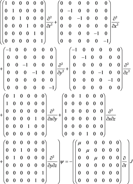
In this appendix we show in details the formulation of Maxwell field equations from the system of linear first order partial differential equations given in Equation (10) of Section 3. The system of equations given in Equation (10) can be written the following matrix form

$\left(A_0\frac{\partial }{\partial t}+A_1\frac{\partial }{\partial x}+A_2\frac{\partial }{\partial y}+A_3\frac{\partial }{\partial z}\right)\psi =A_{4}J$ (1)

where $\psi ={\left({\psi }_1,{\psi }_2,{\psi }_3,{\psi }_4,{\psi }_5,{\psi }_6\right)}^{\text{T}}$,$J={\left(j_1,j_2,j_3,0,0,0\right)}^{\text{T}}$ and the matrices $A_i$ are given as follows

$\begin{array}{l}{A}_0=\left(\begin{array}{cccccc}-1& 0& 0& 0& 0& 0\\ 0& -1& 0& 0& 0& 0\\ 0& 0& -1& 0& 0& 0\\ 0& 0& 0& 1& 0& 0\\ 0& 0& 0& 0& 1& 0\\ 0& 0& 0& 0& 0& 1\end{array}\right),A_1=\left(\begin{array}{cccccc}0& 0& 0& 0& 0& 0\\ 0& 0& 0& 0& 0& -1\\ 0& 0& 0& 0& 1& 0\\ 0& 0& 0& 0& 0& 0\\ 0& 0& -1& 0& 0& 0\\ 0& 1& 0& 0& 0& 0\end{array}\right),\\ A_2=\left(\begin{array}{cccccc}0& 0& 0& 0& 0& 1\\ 0& 0& 0& 0& 0& 0\\ 0& 0& 0& -1& 0& 0\\ 0& 0& 1& 0& 0& 0\\ 0& 0& 0& 0& 0& 0\\ -1& 0& 0& 0& 0& 0\end{array}\right),A_3=\left(\begin{array}{cccccc}0& 0& 0& 0& -1& 0\\ 0& 0& 0& 1& 0& 0\\ 0& 0& 0& 0& 0& 0\\ 0& -1& 0& 0& 0& 0\\ 1& 0& 0& 0& 0& 0\\ 0& 0& 0& 0& 0& 0\end{array}\right),\\ A_4=\left(\begin{array}{cccccc}\mu & 0& 0& 0& 0& 0\\ 0& \mu & 0& 0& 0& 0\\ 0& 0& \mu & 0& 0& 0\\ 0& 0& 0& 0& 0& 0\\ 0& 0& 0& 0& 0& 0\\ 0& 0& 0& 0& 0& 0\end{array}\right)\end{array}$ (2)

The system of equations given in Equation (1) becomes

$-\frac{\partial {\psi }_1}{\partial t}+\frac{\partial {\psi }_6}{\partial y}-\frac{\partial {\psi }_5}{\partial z}=\mu j_1$ (3)

$-\frac{\partial {\psi }_2}{\partial t}+\frac{\partial {\psi }_4}{\partial z}-\frac{\partial {\psi }_6}{\partial x}=\mu j_2$ (4)

$-\frac{\partial {\psi }_3}{\partial t}+\frac{\partial {\psi }_5}{\partial x}-\frac{\partial {\psi }_4}{\partial y}=\mu j_3$ (5)

$\frac{\partial {\psi }_4}{\partial t}+\frac{\partial {\psi }_3}{\partial y}-\frac{\partial {\psi }_2}{\partial z}=0$ (6)

$\frac{\partial {\psi }_5}{\partial t}+\frac{\partial {\psi }_1}{\partial z}-\frac{\partial {\psi }_3}{\partial x}=0$ (7)

$\frac{\partial {\psi }_6}{\partial t}+\frac{\partial {\psi }_2}{\partial x}-\frac{\partial {\psi }_1}{\partial y}=0$ (8)

Using the identification $E=\left({\psi }_1,{\psi }_2,{\psi }_3\right)$ and $B=\left({\psi }_4,{\psi }_5,{\psi }_6\right)$, the above system of equations can be rewritten in the familiar form given in classical electrodynamics as

$\nabla \cdot E=\frac{{\rho }_e}{ϵ}$ (9)

$\nabla \cdot B=0$ (10)

$\nabla \times E+\frac{\partial B}{\partial t}=0$ (11)

$\nabla \times B-ϵ\mu \frac{\partial E}{\partial t}=\mu j_e$ (12)

where the charge density ${\rho }_e$ and the current density $j_e$ satisfy the conservation law

$\nabla \cdot j_e+\frac{\partial {\rho }_e}{\partial t}=0$ (13)

From the matrices $A_i$ given in Equation (2) we obtain

$A_0^2=\left(\begin{array}{cccccc}1& 0& 0& 0& 0& 0\\ 0& 1& 0& 0& 0& 0\\ 0& 0& 1& 0& 0& 0\\ 0& 0& 0& 1& 0& 0\\ 0& 0& 0& 0& 1& 0\\ 0& 0& 0& 0& 0& 1\end{array}\right),A_1^2=\left(\begin{array}{cccccc}0& 0& 0& 0& 0& 0\\ 0& -1& 0& 0& 0& 0\\ 0& 0& -1& 0& 0& 0\\ 0& 0& 0& 0& 0& 0\\ 0& 0& 0& 0& -1& 0\\ 0& 0& 0& 0& 0& -1\end{array}\right),$

$A_2^2=\left(\begin{array}{cccccc}-1& 0& 0& 0& 0& 0\\ 0& 0& 0& 0& 0& 0\\ 0& 0& -1& 0& 0& 0\\ 0& 0& 0& -1& 0& 0\\ 0& 0& 0& 0& 0& 0\\ 0& 0& 0& 0& 0& -1\end{array}\right),A_3^2=\left(\begin{array}{cccccc}-1& 0& 0& 0& 0& 0\\ 0& -1& 0& 0& 0& 0\\ 0& 0& 0& 0& 0& 0\\ 0& 0& 0& -1& 0& 0\\ 0& 0& 0& 0& -1& 0\\ 0& 0& 0& 0& 0& 0\end{array}\right),$

$A_4^2=\left(\begin{array}{cccccc}{\mu }^2& 0& 0& 0& 0& 0\\ 0& {\mu }^2& 0& 0& 0& 0\\ 0& 0& {\mu }^2& 0& 0& 0\\ 0& 0& 0& 0& 0& 0\\ 0& 0& 0& 0& 0& 0\\ 0& 0& 0& 0& 0& 0\end{array}\right),A_1{A}_2+A_2{A}_1=\left(\begin{array}{cccccc}0& 1& 0& 0& 0& 0\\ 1& 0& 0& 0& 0& 0\\ 0& 0& 0& 0& 0& 0\\ 0& 0& 0& 0& 1& 0\\ 0& 0& 0& 1& 0& 0\\ 0& 0& 0& 0& 0& 0\end{array}\right)$

$A_1{A}_3+A_3{A}_1=\left(\begin{array}{cccccc}0& 0& 1& 0& 0& 0\\ 0& 0& 0& 0& 0& 0\\ 1& 0& 0& 0& 0& 0\\ 0& 0& 0& 0& 0& 1\\ 0& 0& 0& 0& 0& 0\\ 0& 0& 0& 1& 0& 0\end{array}\right),A_2{A}_3+A_3{A}_2=\left(\begin{array}{cccccc}0& 0& 0& 0& 0& 0\\ 0& 0& 1& 0& 0& 0\\ 0& 1& 0& 0& 0& 0\\ 0& 0& 0& 0& 0& 0\\ 0& 0& 0& 0& 0& 1\\ 0& 0& 0& 0& 1& 0\end{array}\right)$

$A_0{A}_i+A_i{A}_0=0\text{for}i=1,2,3$ (14)

Now, if we apply the differential operator $\left(A_0\partial /\partial t+A_1\partial /\partial x+A_2\partial /\partial y+A_3\partial /\partial z\right)$ to Equation (1) then we arrive at

(15)

From Equation (15), we obtain the following system of equations for the electric field $E=\left(E_x,E_y,E_z\right)=\left({\psi }_1,{\psi }_2,{\psi }_3\right)$

$\frac{{\partial }^2{\psi }_1}{\partial t^2}-\frac{{\partial }^2{\psi }_1}{\partial y^2}-\frac{{\partial }^2{\psi }_1}{\partial z^2}+\frac{\partial }{\partial x}\left(\frac{\partial {\psi }_2}{\partial y}+\frac{\partial {\psi }_3}{\partial z}\right)=-\mu \frac{\partial j_1}{\partial t}$ (16)

$\frac{{\partial }^2{\psi }_2}{\partial t^2}-\frac{{\partial }^2{\psi }_2}{\partial x^2}-\frac{{\partial }^2{\psi }_2}{\partial z^2}+\frac{\partial }{\partial y}\left(\frac{\partial {\psi }_1}{\partial x}+\frac{\partial {\psi }_3}{\partial z}\right)=-\mu \frac{\partial j_2}{\partial t}$ (17)

$\frac{{\partial }^2{\psi }_3}{\partial t^2}-\frac{{\partial }^2{\psi }_3}{\partial x^2}-\frac{{\partial }^2{\psi }_3}{\partial y^2}+\frac{\partial }{\partial z}\left(\frac{\partial {\psi }_1}{\partial x}+\frac{\partial {\psi }_2}{\partial y}\right)=-\mu \frac{\partial j_3}{\partial t}$ (18)

If the electric field also satisfies Gauss’s law

$\nabla \cdot E=\frac{\partial {\psi }_1}{\partial x}+\frac{\partial {\psi }_2}{\partial y}+\frac{\partial {\psi }_3}{\partial z}=\frac{{\rho }_e}{ϵ}$ (19)

then we obtain the following relations

$\frac{\partial }{\partial x}\left(\frac{\partial {\psi }_2}{\partial y}+\frac{\partial {\psi }_3}{\partial z}\right)=\frac{\partial }{\partial x}\left(\frac{{\rho }_e}{ϵ}-\frac{\partial {\psi }_1}{\partial x}\right)=-\frac{{\partial }^2{\psi }_1}{\partial x^2}+\frac{\partial }{\partial x}\left(\frac{{\rho }_e}{ϵ}\right)$ (20)

$\frac{\partial }{\partial y}\left(\frac{\partial {\psi }_1}{\partial x}+\frac{\partial {\psi }_3}{\partial z}\right)=\frac{\partial }{\partial y}\left(\frac{{\rho }_e}{ϵ}-\frac{\partial {\psi }_2}{\partial y}\right)=-\frac{{\partial }^2{\psi }_2}{\partial y^2}+\frac{\partial }{\partial y}\left(\frac{{\rho }_e}{ϵ}\right)$ (21)

$\frac{\partial }{\partial z}\left(\frac{\partial {\psi }_1}{\partial x}+\frac{\partial {\psi }_2}{\partial y}\right)=\frac{\partial }{\partial z}\left(\frac{{\rho }_e}{ϵ}-\frac{\partial {\psi }_3}{\partial z}\right)=-\frac{{\partial }^2{\psi }_3}{\partial z^2}+\frac{\partial }{\partial z}\left(\frac{{\rho }_e}{ϵ}\right)$ (22)

From Equations (16-18) together with relations given in Equations (20-22), we obtain, in vector form, the wave equation for the electric field as

$\frac{{\partial }^{2}E}{\partial t^2}-{\nabla }^{2}E=\nabla \left(\frac{{\rho }_e}{ϵ}\right)-\mu \frac{\partial J_e}{\partial t}$ (23)

where $J_e=\left(j_1,j_2,j_3\right)$. Similarly for the magnetic field $B=\left(B_x,B_y,B_z\right)=\left({\psi }_4,{\psi }_5,{\psi }_6\right)$ we obtain the following equations and relations

$\frac{{\partial }^2{\psi }_4}{\partial t^2}-\frac{{\partial }^2{\psi }_4}{\partial y^2}-\frac{{\partial }^2{\psi }_4}{\partial z^2}+\frac{\partial }{\partial x}\left(\frac{\partial {\psi }_5}{\partial y}+\frac{\partial {\psi }_6}{\partial z}\right)=0$ (24)

References

- 1. Bransden, B.H. and Joachain, C.J. (1990) Physics of Atoms and Molecules. Longman Scientific & Technical, New York.
- 2. Pons, D.J., Pons, A.D. and Pons, A.J. (2019) Journal of Modern Physics, 10, 835-860. https://doi.org/10.4236/jmp.2019.107056
- 3. Dirac, P.A.M. (1928) Proceedings of the Royal Society A: Mathematical, Physical and Engineering Sciences, 117, 610-624. https://doi.org/10.1098/rspa.1928.0023
- 4. Ho, V.B. (2019) Journal of Modern Physics, 10, 1065-1082. https://doi.org/10.4236/jmp.2019.109069
- 5. Schrödinger, E. (1982) Collected Papers on Wave Mechanics. AMS Chelsea Publishing, New York.
- 6. Bransden, B.H. and Joachain, C.J. (1989) Introduction to Quantum Mechanics. Longman Scientific & Technical, New York.
- 7. Ho, V.B. (2018) Journal of Modern Physics, 9, 2402-2419. https://doi.org/10.4236/jmp.2018.914154
- 8. Newton, I. (1687) The Mathematical Principles of Natural Philosophy. Translated into English by Andrew Motte (1846).
- 9. Einstein, A. (1952) The Principle of Relativity. Dover Publications, New York.
- 10. Ho, V.B. (2017) International Journal of Physics, 6, 105-115. https://doi.org/10.12691/ijp-6-4-2
- 11. Ho, V.B. (2018) Global Journal of Science Frontier Research, 18, 37-58.
- 12. Thaller, B. (1992) The Dirac Equation. Springer-Verlag, New York.
- 13. Strauss, W.A. (1992) Partial Differential Equation. John Wiley & Sons, Inc., New York.
- 14. Ho, V.B. (1994) Journal of Physics A: Mathematical and General, 27, 6237-6241. https://doi.org/10.1088/0305-4470/27/18/031
- 15. Ho, V.B. and Morgan, M.J. (1996) Journal of Physics A: Mathematical and General, 29, 1497-1510. https://doi.org/10.1088/0305-4470/29/7/019
- 16. Ho, V.B. (1996) Geometrical and Topological Methods in Classical and Quantum Physics. PhD Thesis, Monash University, Clayton.
- 17. Ho, V.B. (2018) Fluid State of the Electromagnetic Field.