American Journal of Operations Research
Vol. 2 No. 2 (2012) , Article ID: 19935 , 10 pages DOI:10.4236/ajor.2012.22022
Immune Optimization Approach for Dynamic Constrained Multi-Objective Multimodal Optimization Problems*
Institute of System Science & Information Technology, College of Science, Guizhou University, Guiyang, China
Email: sci.zhzhang@gzu.edu.cn
Received March 13, 2012; revised April 15, 2012; accepted April 30, 2012
Keywords: Dynamic Constrained Multi-Objective Optimization; Multimodality; Artificial Immune Systems; Immune Optimization; Environmental Detection
ABSTRACT
This work investigates one immune optimization approach for dynamic constrained multi-objective multimodal optimization in terms of biological immune inspirations and the concept of constraint dominance. Such approach includes mainly three functional modules, environmental detection, population initialization and immune evolution. The first, inspired by the function of immune surveillance, is designed to detect the change of such kind of problem and to decide the type of a new environment; the second generates an initial population for the current environment, relying upon the result of detection; the last evolves two sub-populations along multiple directions and searches those excellent and diverse candidates. Experimental results show that the proposed approach can adaptively track the environmental change and effectively find the global Pareto-optimal front in each environment.
1. Introduction
In real-world engineering problems, a great number of optimization problems often involve in multiple timevarying multimodal sub-objectives and constraints, such as portfolio investment, project planning management, chemical engineering design and transportation. These belong to dynamic constrained multi-objective multimodal optimization (DCMMO) which the sub-objective functions, constraints, dimensions of the objective space and design space may change over time. The major challenge lies in that the global Pareto front may move toward another one with time; it is very difficult for a search procedure to keep the sufficient diversity and convergence, due to multiple local Pareto fronts and constraints. Although some techniques are popular in the context of intelligent optimization, they expose many faults when directly applied to DCMMO problems, e.g., adaptation, genetic diversity and constraint-handling. Dynamic multi-objective optimization (DMO) has become active in the recent years. Many researchers in the fields of evolutionary computation and immune optimization have made their efforts to study how the search procedure can adaptively track the environmental change and rapidly find the desired Pareto front [1-10]. DCMMO is one particular kind of DMO, presenting complex dynamic behaviors such as dynamics and multimodality. In order to solve such special kind of problem, we must solve at least three crucial issues: 1) infeasible individuals toward feasible ones, 2) population diversity, and (3) finding the well-distributed global Pareto front.
Although immune optimization, a popular research branch, was proved to be potential for dynamic problems because of the inherent diversity and adaptation, more studies on it are concentrated on solving non-constrained dynamic single or multi-objective optimization problems [10-12]. It is not clear whether bio-immune inspirations are valuable for handling DCMMO. To our knowledge, it is possible to explore efficient and effective immune techniques for such kind of problem. Thereby, we in the present work try studying an immune-inspired optimization approach, dynamic constrained multi-objective multimodal immune optimization approach (DCMMIOA). The comparative experiments draw the strong conclusion that DCMMIOA is a competitive optimizer capable of rapidly tracking the environmental change and effectively discovering the location of the global Pareto front in each environment.
2. Related Work Survey on Intelligent Optimization for DMO
2.1. Dynamic Multi-Objective Evolutionary Algorithms
DMO has recently gained great attention among researchers in the area of intelligent optimization. The key of designing an advanced technique for such problem is to consider such crucial factors as computational complexity, environmental adaptation and solution quality. Several researchers [1-7] have reported their excellent achievements suitable for non-constrained DMO problems. For example, Farina, et al. [1] constructed five dynamic multi-objective test problems with slowly changing environments and fixed dimensions, based on the static benchmark test problems; meanwhile, one-directional search-based method was proposed to solve them. This method can obtain some Pareto-optimal solutions with somewhat uniform distribution for a given problem, but time consumption is expensive. In [2], two similar dynamic optimization techniques originating from NSGAII, i.e., DNSGAII-A and DNSGAII-B, were proposed to find a minimum frequency of change allowed in the problem to adequately track the theoretical Pareto front on-line. Their main difference is only with the aspect of generating their respective initial populations. One of their merits is that they can also solve DCMO problems. In the DMO studies done by Zhou and Hatzakis [4,5], some prediction-based inspirations were merged into one reported multi-objective evolutionary algorithm, in which the time serial analysis method was used to predict the location of the Pareto front. In addition, in the work made by Wang [6], a new evolutionary algorithm (DMEA) was proposed to deal with DCMO problems, by improving the operators of crossover and mutation. In a study done by Tan [7], one competitive and cooperative mechanisms-based co-evolutionary multi-objective algorithm was developed to solve multi-objective optimization problems in dynamic environments. For one such algorithm, each species subpopulation competes to represent a particular subcomponent of the multi-objective problem, while the eventual winners are required to coevolve so that those better solutions can be found.
2.2. Dynamic Multi-Objective Immune Optimization (DMIO)
Since Carlos et al. proposed a simple artificial immune system to solve static multi-objective optimization problems [13,14], multi-objective immune optimization has become increasingly active. Correspondingly, many original or improved immune techniques [15-17], based on the humoral immune response principle, have been reported continually. This indicates that the artificial immune system paradigm is an interesting topic for multiobjective optimization problems. However, less work on DMIO is displayed in the literature. Shang et al. [8] suggested one clonal selection algorithm for dynamic nonconstrained multi-objective optimization problems, while such approach was examined by two theoretical test problems. More recently, we also studied immune-based optimization techniques for such kind of problem [9]. Subsequently, we handled one general kind of DCMO by developing an immune agent-based artificial immune system (DCMOAIS) [10]. In this approach, the interactive mechanism between B-cell and T-cell is our major bio-inspiration. The experimental results hint that such approach is a competitive optimizer for complex and high-dimensional DCMO problems. Despite of some reported achievements on DMIO, they might be difficult in solving multimodal optimization problems. Thereby, we in this work design DCMMIOA to solve specially DCMMO problems rather than general DCMO. It should be pointed out that although DCMMIOA and DCMOAIS share some bio-immune inspirations, their modules are completely different. For example, DCMMIOA does not include memory pool, while detecting the environmental change only by means of the joint environment; it carries out evolution on two sub-populations, in which the better subpopulation executes multiple evolution schemes so that some global Pareto-optimal solutions can be found.
3. Problem Formulation and Immune Theory
3.1. Problem Formulation
Consider the dynamic constrained multi-objective multimodal optimization problem (VP):

with discrete time integer variable t,  , and bounded and closed domain
  in
in , where n(t) is the dimension at the moment
 ;
;  denotes the time-varying vector-valued objective function with at least one multimodal sub-objective function; gi(x,t),
  , are the linear or nonlinear inequality constraint functions. Since t takes integers in the interval [1, T], the above problem consists of a series of jointly static multiobjective multimodal problems; each static problem is called an environment; for example, we call the t-th static problem the t-th environment. Our task is to develop DCMMIOA which can continually track the environmental change and rapidly search the global Pareto front in the t-th environment before the next environment arrives.
Additionally,  is said to be feasible for the t-th environment, if it satisfies all the above constraints, and infeasible otherwise. For a given environment t and
 , we say that x constrained-dominates y if one of three conditions is true [2]: (1) x is feasible but y is not; (2) x and y are feasible and
 ; (3) x and y are both infeasible, but x has a smaller constraint violation
 . Here,
  denotes that fl(x,t) ≤ fl(y,t), 1 ≤ l ≤ m, and there exists j, 1 ≤ j ≤ m, such that fj(x,t) < fj(y,t); meanwhile,
  represents the total of constraint violations at the point x for all the constraints; namely,
  is the sum of
  with
with . For a given environment t,
  is called a local Pareto-optimal solution, if it is feasible, and there exists a neighborhood in x such that any element in such region does not constrained-dominate x;
  is said to be a global Pareto-optimal solution, if it is feasible, and all elements in
  do not constrained-dominate x.
3.2. Immune Theory
The immune response theory describes essentially a process that B and T cells learn an invader and ultimately eliminate it. T cells as detectors can monitor whether a change takes place in the immune system, being capable of identifying “self” and “non-self”. When an organism is attacked by the invader or antigen, T cells will experience three phases: initiation, reaction and elimination; namely, a large number of virgin cells are first generated, and then these cells become effectors which urge B cells to respond to the antigen. This stimulates these B cells to create plasma and memory cells through proliferation. If being active, such plasma cells suffer a process of affinity maturation through somatic maturation, and secrete antibodies neutralizing the triggering invader. Subsequently, high-affinity B cells are selected into the B-cell pool, but others are eliminated. Besides, the memory cells will become long-lived ones. Once the previous invader is found in the immune system, these memory cells commence rapidly differentiating into plasma cells capable of producing high-affinity antibodies.
Summarily, by taking an analogy between the two processes of the immune response and solving DCMMO, it is not difficult to know that the task of such response is to create excellent B cells and the purpose of handling DCMMO is to find those best solutions. From the viewpoint of engineering application, such immune response is a bio-inspiration used in developing immune-inspired optimizers. In this work, two immune metaphors of Tcell surveillance and B-cell learning (cell selection, clonal expansion and somatic mutation) are simply simulated to construct our DCMMIOA. The first is adopted to design the module of environmental detection which detects the environmental change; the second is an important biological idea used to create valuable B cells or individuals.
4. Algorithm Formulation and Module Illustration
4.1. Algorithm Formulation
As associated to problem (VP) as in Section 3, for the t-th environment antigen  is viewed as the attribute set of
 ,
,  and
and , where
  is the vector-valued function composed of constraint functions; B cells are regarded as real-encoded candidate solutions; memory cells denotes those best B cells found until now (i.e., non-dominated candidates). DCMMIOA includes five modules of environmental detection, initialization, division, mutation and recruitment. Following these descriptions, it can be in detail described as follows.
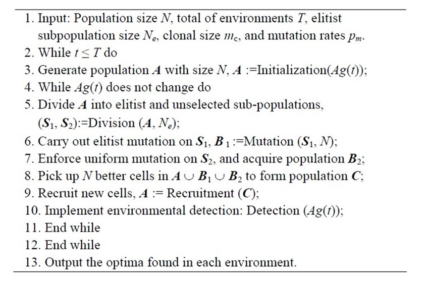
Notice that in the above approach, steps 4 to 11 is a loop of optimization for the t-th environment. Through step 10, once such environment takes a change, the search process in the environment is required to stop. Steps 6 and 7 formulate two sub-populations to evolve along different directions. Additionally, some optimization problems usually include multiple constraints so that their feasible regions are empty or extremely narrow. In such case, it becomes difficult for any optimization approach to solve them. Thus, when handling this kind of hardconstraint problem, the requirement of feasibility is relaxed. Here, we design a threshold index to decide whether an individual is feasible or not, namely
 (1)
(1)
where n and Mn(t) denote the iteration number and the maximal iteration in the t-th environment, respectively. If , we say that x is feasible. The main modules are designed below.
4.2. Module Illustration
Detection (Ag(t)). This module detects whether Ag(t) has made a change within the runtime, and decides the relation between Ag(t) and Ag(t + 1) if so. Note that Ag(t) comprises of three factors, i.e., n(t), f(., t) and . If any change takes place among such three factors, we say that the t-th environment has changed. Suppose that such environment has been converted to environment t + 1; so, we decide whether Ag(t + 1) is new or similar through the following way:
1) If , Ag(t + 1) is regarded as a new antigen;
2) If , we pick randomly up K cells in the eventual population A acquired in the t-th environment to constitute a sample set S, and then check the relation between Ag(t) and Ag(t + 1) through an identification factor
 defined as
 (2)
(2)
where  stands for the 2-norm of x. If
 , we say that Ag(t + 1) is similar to Ag(t); otherwise, Ag(t + 1) is new. Here, we take
 .
.
Initialization (Ag(t)) includes N cells decided through the type of Ag(t). More precisely, if Ag(t) is new, such N cell are generated randomly; otherwise, some random B cells and  of elements from the eventual population gotten in the last environment constitute the initial population. Here, we take
 .
.
Division (A, Ne) consists of two sub-populations S1 and S2, where each element in S1 is superior to any one in S2. Precisely, relying upon the concept of constraintdominance, population A is first sorted orderly into non-dominated classes F1, F2, ··· ,Fl, where the first is best and the last is worst. Suppose that F1 involves in np members. If np < Ne, pick up some elements in F2 with small concentrations, together with those in F1, to constitute S1, where the concentration of x in F2, C(x), is decided by
 . (3)
. (3)
Note that |A| denotes the number of elements in A, and we in this work take . If
. If , go on this process by substituting F3 for F2 in Equation (3), until that S1 includes Ne elements. If np > Ne, the conventional crowding distance approach, proposed by Deb et al. [2], is applied to F1, and selects Ne elements with large crowding distances to form S1. Further, S2 consists of those elements in A but not in S1.
Mutation (S1, N) comprises of new B cells acquired through multiple mutation fashions on S1. To this end, considering exploitation and exploration, we carry out a np-dependent mutation, where np is mentioned above. Namely, we first copy ξN better elements in S1 to proliferate their clones with respectively clonal sizes mc; each of clones undergoes the following Gaussian mutation with the mutation probability pm,
 (4)
(4)
with variance ξβ, where γ is a randomly generated number in (0, 1), and we take ξ = 0.1 in this paper. Further, for a pre-defined threshold λ with 0 < λ < 1, if np < λN, each B cell in S1 changes its genes with the mutation probability , relying upon Equation (4) but with variance
 ; otherwise, if a randomly generated number
  in (0, 1) satisfies
 , each element in S1 shifts its genes as in the case of np < λN but with the variance
 , and conversely, each B cell is mutated with the mutation probability pm through
 (5)
(5)
where r and r1 are both randomly generated values in (0, 1). After the three mutation fashions are completed, all mutated cells constitute a new subpopulation B1.
Recruitment (C) includes those better cells in C and some new ones obtained through crossover. That is, take η% of the worse elements in C to interact with B cells randomly selected in the above best subclass F1, through crossover and with the crossover probability 1. After so, those new cells, together with the better cells in C, constitute the desired population A.
5. Performance Criteria
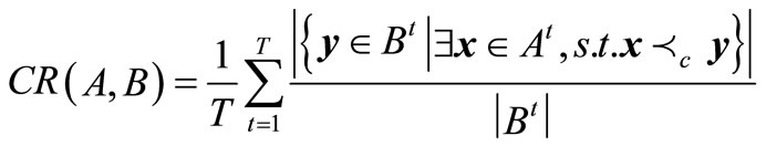
To measure DCMMIOA’s performance, several evaluation criteria are developed through extending the three conventional criteria [20], i.e., coverage rate (CR), coverage density (CD) and coverage scope (CS). If two algorithms A and B are executed respectively a single run in each of the T environments as in problem (VP) above, two series of non-dominated sets are acquired,  and
and .
.
(A) coverage rate. This can be used to compare the qualities of non-dominated solutions gotten by algorithms A and B, given by
 (6)
(6)
Equation (6) shows that the non-dominated sets found by algorithm A are globally better than those gained by algorithm B if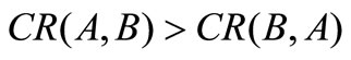 .
.
(B) coverage density and scope. Coverage density CD is utilized to measure the whole distribution of the non-dominated solutions obtained by algorithm A in the environments, defined as
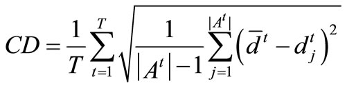 (7)
(7)
where
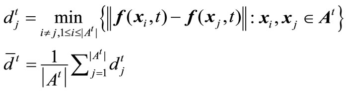
Equation (7) hints that the smaller the value CD, the better the distribution of the non-dominated solutions. Similarly, coverage scope is denoted by the average coverage width of solutions acquired in the environments, given by
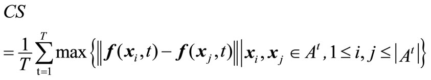 (8)
(8)
Obviously, Equation (8) shows that a larger value of CS means a wider coverage scope of the solutions.
6. Experimental Study
In this section, we execute all experiments on a computer with CPU/3.0 GHz and RMB/2.0 GB. In order to test DCMMIOA’s characteristics, three dynamic constrained multi-objective evolutionary algorithms reported are selected to compare against it, i.e., DMEA [6] and two similar versions of DNSGAII-A and DNSGAII-B [2]. In addition, we give seven DCMO problems DCTP1 to DCTP7 acquired by introducing a time-varying Rastrigin function into the seven static benchmark problems CTP1 to CTP7 [18], and two dynamic engineering design problems DSR and DPVM gained through modifying the coefficients of the two original versions [19,20]; more details can be found below. Such dynamic problems are utilized to examine the inherent properties of these four approaches.
To analyze fairly the performance characteristics of the above algorithms, each approach with population size 100 is admitted to execute 30 single runs on each test problem, and evaluates 105 times in each environment for DCTP6, DSR and DPVM but 50,000 times for other test problems. Take four environments for each test problem. The other parameter settings of the three compared algorithms can be known through their corresponding references. For DCMMIOA, we take mc = 5, pm = 0.3, Ne = 50, α = 2.0 for all the test problems; we set λ = 0.8, β = 0.1 for problems DCTP1 to DCTP5, DCTP7 and DSR, take λ = 0.4, β = 2.0 for DCTP6, and set λ = 0.8, β = 2 for DPVM.
6.1. Benchmark Problems and Experimental Analysis
Deb et al. designed a series of static constrained multiobjective test problems, i.e., CTP1 to CTP7 [18]. We modify their common function g(x) into the following time-varying Rastrigin’s multimodal function,
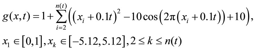
and correspondingly, the static problems are extended in order into dynamic multi-objective multimodal problems DCTP1 to DCTP7. For either DCTP1 or DCTP7, the four environments are with dimensions 10, 10, 12 and 12 in turn, but 10, 10, 10 and 10 for each other problem. Depending on the performance criteria as in section 5, we obtain the statistical results in Table 1 below, and the non-dominated fronts, found by such algorithms with respectively a single run, are presented in Figure 1 below. In Table 1, A1, A2, A3 and A4 stand for DNSGAIIA, DNSGAII-B, DMEA and DCMMIOA, respectively.
Relying upon Table 1 and Figure 1, DCMMIOA spends the least average runtime to solve all the test problems except DCTP4 and DCTP7, and DMEA is secondary. We also notice that DNSGAII-A and DNSGAII-B demand globally more time to deal with the above problems.
The average coverage rates (ACR) illustrate clearly that DCMMIOA’s optimized quality for each of the above problems is globally best, as the qualities of the non-dominated solutions found by it in each environment are globally better than those gotten by any of the other algorithms for each problem, e.g., for DCTP1, the nondominated sets acquired by DCMMIOA in each environment cover averagely 38%, 40% and 90% of those obtained by DNSGAII-A, DNSGAII-B and DMEA, respectively; conversely, the non-dominated solutions acquired by the latter three algorithms in each environment dominate in order only 6%, 6% and 1% of those found by DCMMIOA. This shows that DCMMIOA, with a rational balance between convergence and diversity, can effectively track the global Pareto front in each environment per problem. In addition, Figure 1 hints that once the environment become severe, DNSGAII-B and DMEA degrade seriously their performances; in particular, they can only acquire the local Pareto fronts (see Figures 1((a), (f) and (g)). Further, we note that only DCMMIOA can track the time-varying global Pareto front for DCTP6 (see Figure 1(f)), which shows that those compared algorithms get easily into local search and hence expose their weak diversity. The statistical values on CS present that each non-dominated set found by DCMMIOA in each environment for each problem has the globally wider coverage scope than that acquired by any of other algorithms, which indicates that such approach can find those excellent and diverse non-dominated solutions. In addition, the statistical values on CD show that these


Table 1. Statistical comparison of non-dominated sets found for problems DCTP1 to DCTP7.
 (a)
(a) (b)
(b)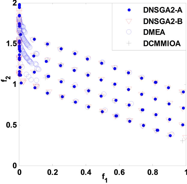 (c)
(c)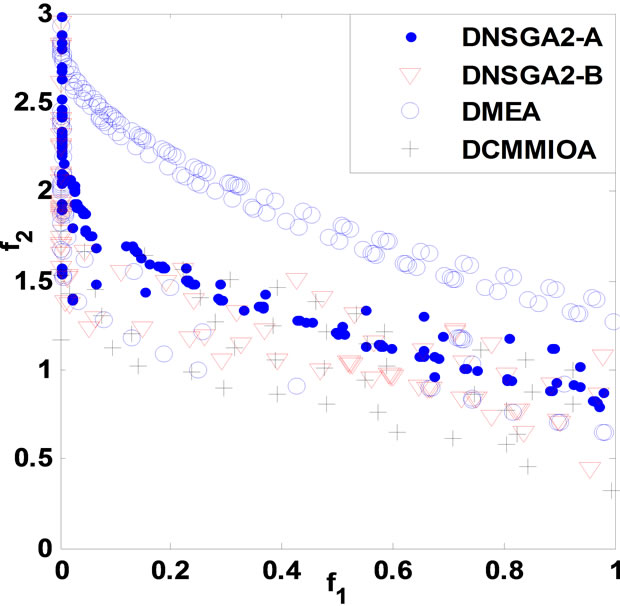 (d)
(d)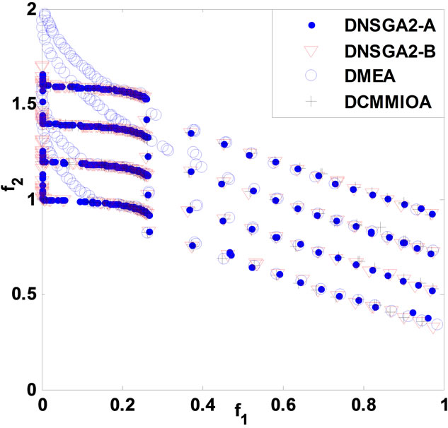 (e)
(e) (f)
(f) (g)
(g)
Figure 1. Comparison of non-dominated fronts obtained by the four algorithms in each environment. (a) DCTP1; (b) DCTP2; (c) DCTP3; (d) DCTP4; (e) DCTP5; (f) DCTP6; (g) DCTP7.
approaches can effectively eliminate those similar nondominated solutions, and thereby their resultant solutions are with the satisfactory distribution. Summarily, through the statistical values on ACR, CS and CD, we can clearly see that DCMMIOA acquires the best solution quality for each test problem while DNSGAII-A is secondary.
Totally, for each test problem above, we can draw the strong conclusion that DCMMIOA performs well over the compared approaches; DMEA has the higher efficiency than either DNSGAII-A or DNSGAII-B, but the worse effect than DNSGAII-A.
6.2. Experimental Results on Engineering Problems
We take the dynamic speed reducer model (DSR) for example. Such model can be found in [19]. Similar to the above experiment, the above algorithms get their statistical results given in Table 2, and the non-dominated fronts are drawn in Figure 2. Note that since DMEA fails to solve such model, we do not give its statistical results.
Table 2 and Figure 2 display the results obtained by DNSGAII-A, DNSGAII-B and DCMMIOA for problem DSR. We know easily that DCMMIOA has the prominent superiority over two other algorithms, because the non-dominated sets obtained by it cover 96% of those found by either DNSGAII-A or DNSGAII-B, i.e., ACR (A4, A1) = 96%, ACR(A4, A2) = 96%. Further, from other statistical values, we observe that in each environment, DCMMIOA can find some non-dominated solutions with the wide coverage and satisfactory distribution. On the other hand, we see that the solutions found by DNSGAIIA and DNSGAII-B have the similar distribution and coverage. Further, it is obvious that DCMMIOA has the high efficiency when solving the above problem, but the compared approaches cause the slow searching behaviors. Totally, DCMMIOA performs best for this problem, and DNSGAII-B is slightly better than DNSGAII-A.
We next solve the other engineering problem, Dynamic Pressure Vessel Model (DPVM). The static pressure vessel model is proposed originally by Deb and Srinivasan [20]. It aims to minimize the cost of fabrication and to maximize the storage capacity of the vessel, and includes four variables, i.e., thickness of cylindrical part of the vessel ( ), the hemispherical heads (
 ), radius of vessel (
 ) and length of vessel (
 ). We convert it into a dynamic model through modifying the parameter settings. DPVM is formulated as follow:
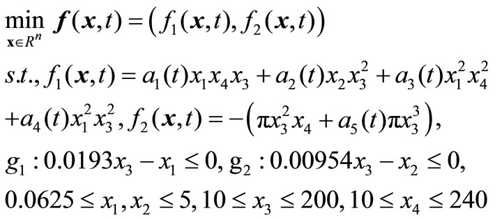
where the coefficients ,
,  , are acquired by introducing time-varying parameters,

Similar to the process of solving the above problems, the algorithms obtain their statistical results for DPVM given in Table 3, and their non-dominated fronts are presented in Figure 3 below.
Through Table 3 and Figure 3, we notice that although DMEA behaves worst, it can obtain some feasible solutions in each environment. Besides, we can obtain the same conclusion as that given in DSR; namely, by comparison to either DNSGAII-A or DNSGAII-B, DCMMIOA has the best optimized quality and the higher performance efficiency; DNSGAII-A and DNSGAII-B present similar effects and almost equal efficiencies. On the other hand, we also see that the non-dominated sets found by DNSGAII-A, DNSGAII-B and DCMMIOA are with similar distributions and coverage scopes, but there are some subtle differences between them. DCMMIOA can globally achieve stable search performance, due to the small variances on CD and CS. Therefore, for the
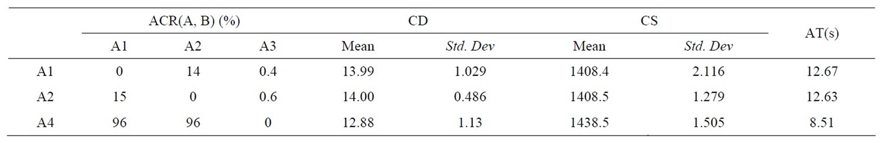
Table 2. Comparison of statistical values obtained for DSR.
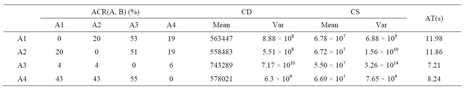
Table 3. Comparison of statistical values obtained by the four algorithms for problem DPVM.

Figure 2. Comparison of non-dominated fronts obtained in each environment for DSR.
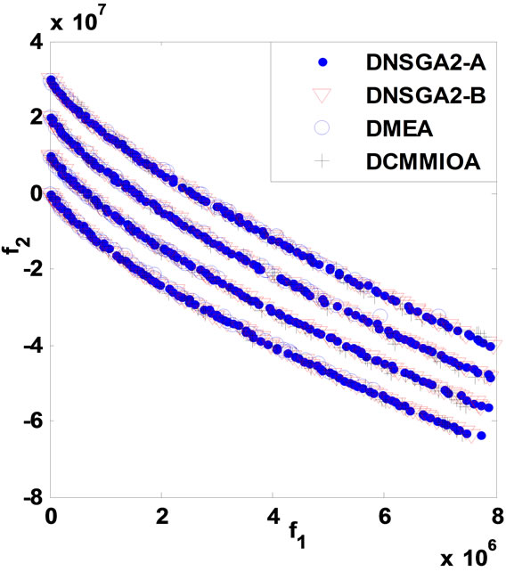
Figure 3. Comparison of non-dominated fronts obtained in each environment for DPVM.
above problem, DCMMIOA performs best, and DNSGAIIA and DNSGAII-B are secondary.
7. Conclusion
DCMMO is an extremely challenging research topic in the field of optimization, due to multimodality. We in this paper investigate such topic because of the increasing requirement of real-world multimodal optimization problems. Correspondingly, one bio-immune optimization approach, inspired by the immune surveillance and interactive metaphors between B cells, is developed to adapt dynamically to the environmental change and to find the global Pareto optimal solutions in each environment. Such approach can adaptively monitor the complex environment and find multiple valuable regions. The experimental results show that it outperforms the compared algorithms and is potential for DCMMO problems; in other word, it can efficiently track the dynamic environment and keep the sufficient diversity, while being capable of approaching the global Pareto front in each environment.
REFERENCES
- M. Farina, K. Deb and P. Amato, “Dynamic Multi-Objective Optimization Problems: Test Case, Approximations, and Applications,” Evolutionary Computation, Vol. 8, No. 5, 2004, pp. 425-442. doi:10.1109/TEVC.2004.831456
- K. Deb, B. R. N. Udaya and S. Karthik, “Dynamic MultiObjective Optimization and Decision-Making Using Modified NSGA-II: A Case Study on Hydro-Thermal Power Scheduling Bi-Objective Optimization Problems,” Lecture Notes in Computer Science, Vol. 4403, 2007, pp. 803-817. doi:10.1007/978-3-540-70928-2_60
- J. Mehnen, T. Wagner and G. Rudolph, “Evolutionary Optimization of Dynamic Multi-Objective Test Functions,” Proceedings of the Second Italian Workshop on Evolutionary Computation, Siena, September 2006.
- A. Zhou, Y. C. Jin, Q. Zhang, B. Sendhoff and E. Tsang, “Prediction-Based Population Re-Initialization for Evolutionary Dynamic Multi-Objective Optimization,” The Fourth International Conference on Evolutionary MultiCriterion Optimization, Matsushima, 5-8 March 2007, pp. 832-846.
- I. Hatzakis and D. Wallace, “Dynamic Multi-Objective Optimization with Evolutionary Algorithms: A ForwardLooking Approach,” Proceedings of the 8th Annual Conference on Genetic and Evolutionary Computation, Seattle, Washington, 2006, pp. 1201-1208.
- C. A. Liu and Y. P. Wang, “Multi-Objective Evolutionary Algorithm for Dynamic Nonlinear Constrained Optimization Problems,” Systems Engineering and Electronics, Vol. 20, No. 1, 2009, pp. 204-210.
- K. C. Tan, “A Competitive-Cooperative Coevolutionary Paradigm for Dynamic Multi-Objective Optimization,” IEEE Transactions on Evolutionary Computation, Vol. 13, No. 1, 2009, pp. 103-127. doi:10.1109/TEVC.2008.920671
- R. H. Shang, L. C. Jiao, M. G. Gong and B. Lu, “Clonal Selection Algorithm for Dynamic Multi-Objective Optimization,” In: Y. Hao, et al., Eds., Computational Intelligence and Security, Springer, Berlin, Heidelberg, Vol. 3801, 2005, pp. 846-851. doi:10.1007/11596448_125
- Z. H. Zhang, “Multi-Objective Optimization Immune Algorithm in Dynamic Environments and Its Application to Greenhouse Control,” Applied Soft Computing, Vol. 8, No. 2, 2008, pp. 959-971. doi:10.1016/j.asoc.2007.07.005
- Z. H. Zhang and S. Q. Qian, “Artificial Immune System in Dynamic Environments Solving Time-Varying NonLinear Constrained Multi-Objective Problems,” Soft Computing, Vol. 15, No. 7, 2011, pp. 1333-1349. doi:10.1007/s00500-010-0674-z
- E. Hart and J. Timmis, “Application Areas of AIS: The Past, Present and the Future,” Applied Soft Computing, Vol. 8, No. 1, 2008, pp. 191-201. doi:10.1016/j.asoc.2006.12.004
- J. Timmis, P. Andrews and E. Hart, “On Artificial Immune Systems and Swarm Intelligence,” Swarm Intelligence, Vol. 4, No. 4, 2010, pp. 247-273. doi:10.1007/s11721-010-0045-5
- C. A. Coello Coello and N. Cruz Cortés, “An Approach to Solve Multi-Objective Optimization Problems Based on an Artificial Immune System,” In: J. Timmis and P. J. Bentley, Eds., First International Conference on Artificial Immune Systems, Canterbury, 2002, pp. 212-221.
- N. Cruz Cortés and C. A. Coello Coello, “Using Artificial Immune Systems to Solve Optimization Problems,” Workshop Program of Genetic and Evolutionary Computation Conference, 2003, pp. 312-315.
- I. Aydin, M. Karakose and E. Akin, “A Multi-Objective Artificial Immune Algorithm for Parameter Optimization in Support Vector Machine,” Applied Soft Computing, Vol. 11, No. 1, 2011, pp. 120-129. doi:10.1016/j.asoc.2009.11.003
- Z. H. Hu, “A Multiobjective Immune Algorithm Based on a Multiple-Affinity Model,” European Journal of Operational Research, Vol. 202, No. 1, 2010, pp. 60-72. doi:10.1016/j.ejor.2009.05.016
- J. Q. Gao and J. Wang, “WBMOAIS: A Novel Artificial Immune System for Multi-Objective Optimization,” Computers & Operations Research, Vol. 37, No. 1, 2010, pp. 50-61. doi:10.1016/j.cor.2009.03.009
- K. Deb, A. Pratap, and T. Meyarivan, “Constrained Test Problems for Multi-Objective Evolutionary Optimization,” Evolutionary Multi-Criterion Optimization Lecture Notes in Computer Science, Vol. 1993, 2001, pp. 284- 298.
- A. Kurpati, S. Azarm and J. Wu, “Constraint Handling Improvements for Multiobjective Genetic Algorithms,” Structural Multidisciplinary Optimization, Vol. 23, No. 3, 2002, pp. 204-213. doi:10.1007/s00158-002-0178-2
- K. Deb and A. Srinivasan, “Monotonicity Analysis, Evolutionary Multi-Objective Optimization, and Discovery of Design Principles,” Indian Institute of Technology, Kanpur Genetic Algorithm Laboratory (KanGAL), Report No. 2006004, 2006.
NOTES
*This research is supported by National Natural Science Foundation NSFC (61065010)